Page 636 - Krugmans Economics for AP Text Book_Neat

produce at point E in Figure 59.2, corresponding to an output of 5 bushels. Note that
The short-run individual supply curve
point C in Figure 59.2 corresponds to the farm’s break-even price of $14 per bushel.
shows how an individual firm’s profit-
Since E lies above C, Jennifer and Jason’s farm will be profitable; they will generate a
maximizing level of output depends on the
per-bushel profit of $18.00 − $14.40 = $3.60 when the market price is $18.
market price, taking fixed cost as given.
But what if the market price lies between the shut-down price and the break-even
price—that is, between the minimum average variable cost and the minimum average
total cost? In the case of Jennifer and Jason’s farm, this corresponds to prices anywhere
between $10 and $14—say, a market price of $12. At $12, Jennifer and Jason’s farm is
not profitable; since the market price is below the minimum average total cost, the
farm is losing (on average) the difference between price and average total cost on every
unit produced. Yet even though the market price isn’t covering Jennifer and Jason’s av-
erage total cost, it is covering their average variable cost and some—but not all—of the
average fixed cost. If a firm in this situation shuts down, it will incur no variable cost
but it will incur the full fixed cost. As a result, shutting down will generate an even
greater loss than continuing to operate.
This means that whenever price falls between minimum average total cost and min-
imum average variable cost, the firm is better off producing some output in the short
run. The reason is that by producing, it can cover its variable cost and at least some of
its fixed cost, even though it is incurring a loss. In this case, the firm maximizes profit—
that is, minimizes loss—by choosing the quantity of output at which its marginal cost
is equal to the market price. So if Jennifer and Jason face a market price of $12 per
bushel, their profit-maximizing output is given by point B in Figure 59.2, correspon-
ding to an output of 3.5 bushels.
It’s worth noting that the decision to produce when the firm is covering its variable
cost but not all of its fixed cost is similar to the decision to ignore a sunk cost, a concept
we studied previously. You may recall that a sunk cost is a cost that has already been
incurred and cannot be recouped; and because it cannot be changed, it should have no
effect on any current decision. In the short-run production decision, fixed cost is, in
effect, like a sunk cost—it has been spent, and it can’t be recovered in the short run.
This comparison also illustrates why variable cost does indeed matter in the short
run: it can be avoided by not producing.
And what happens if the market price is exactly equal to the shut-down price, the
minimum average variable cost? In this instance, the firm is indifferent between pro-
ducing 3 units or 0 units. As we’ll see shortly, this is an important point when looking
at the behavior of an industry as a whole. For the sake of clarity, we’ll assume that the
firm, although indifferent, does indeed produce output when price is equal to the
shut-down price.
Putting everything together, we can now draw the short-run individual supply
curve of Jennifer and Jason’s farm, the red line in Figure 59.2; it shows how the profit-
maximizing quantity of output in the short run depends on the price. As you can see,
the curve is in two segments. The upward-sloping red segment starting at point A
shows the short-run profit-maximizing output when market price is equal to or above
the shut-down price of $10 per bushel. As long as the market
price is equal to or above the shut-down price, Jennifer and Jason
will produce the quantity of output at which marginal cost is
equal to the market price. So at market prices equal to or above
the shut-down price, the firm’s short-run supply curve corre-
sponds to its marginal cost curve. But at any market price below
the minimum average variable cost, in this case, $10 per bushel—
the firm shuts down and output drops to zero in the short run.
This corresponds to the vertical segment of the curve that lies on
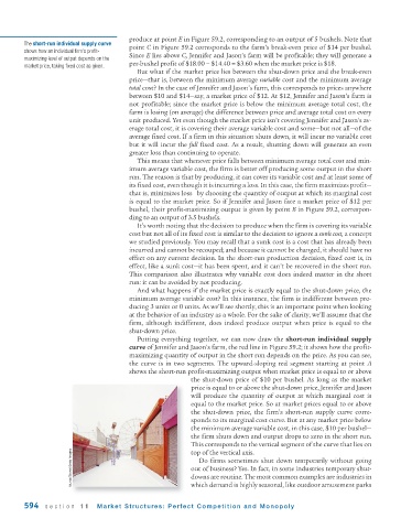
Muntz/Stone/Getty Images out of business? Yes. In fact, in some industries temporary shut-
top of the vertical axis.
Do firms sometimes shut down temporarily without going

downs are routine. The most common examples are industries in
which demand is highly seasonal, like outdoor amusement parks

594 section 11 Market Structures: Perfect Competition and Monopoly