Page 767 - Krugmans Economics for AP Text Book_Neat

about pollution? However, pollution avoidance requires the use of money and inputs
The socially optimal quantity of
that could otherwise be used for other purposes. For example, to reduce the quantity of
pollution is the quantity of pollution that
sulfur dioxide they emit, power companies must either buy expensive low-sulfur coal or society would choose if all the costs
install special scrubbers to remove sulfur from their emissions. The more sulfur diox- and benefits of pollution were fully
ide they are allowed to emit, the lower are these avoidance costs. If we calculated how accounted for.
much money the power industry would save if it were allowed to emit an additional ton
of sulfur dioxide, that savings would be the marginal benefit to society of emitting that
ton of sulfur dioxide.
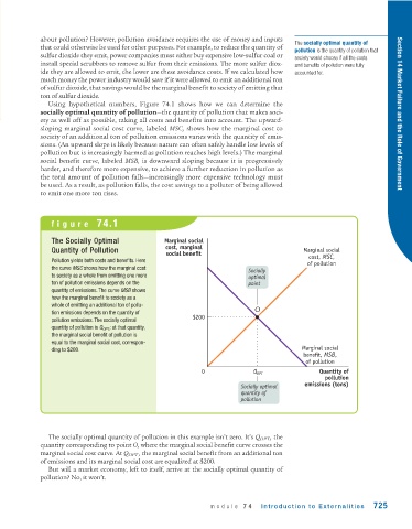
Using hypothetical numbers, Figure 74.1 shows how we can determine the
socially optimal quantity of pollution—the quantity of pollution that makes soci- Section 14 Market Failure and the Role of Government
ety as well off as possible, taking all costs and benefits into account. The upward-
sloping marginal social cost curve, labeled MSC, shows how the marginal cost to
society of an additional ton of pollution emissions varies with the quantity of emis-
sions. (An upward slope is likely because nature can often safely handle low levels of
pollution but is increasingly harmed as pollution reaches high levels.) The marginal
social benefit curve, labeled MSB, is downward sloping because it is progressively
harder, and therefore more expensive, to achieve a further reduction in pollution as
the total amount of pollution falls—increasingly more expensive technology must
be used. As a result, as pollution falls, the cost savings to a polluter of being allowed
to emit one more ton rises.

figure 74.1

The Socially Optimal Marginal social
Quantity of Pollution cost, marginal Marginal social
social benefit cost, MSC,
Pollution yields both costs and benefits. Here of pollution
the curve MSC shows how the marginal cost
Socially
to society as a whole from emitting one more optimal
ton of pollution emissions depends on the point
quantity of emissions. The curve MSB shows
how the marginal benefit to society as a
whole of emitting an additional ton of pollu-
tion emissions depends on the quantity of $200 O
pollution emissions. The socially optimal
quantity of pollution is Q OPT ; at that quantity,
the marginal social benefit of pollution is
equal to the marginal social cost, correspon-
ding to $200. Marginal social
benefit, MSB,
of pollution
0 Q OPT Quantity of
pollution
emissions (tons)
Socially optimal
quantity of
pollution

The socially optimal quantity of pollution in this example isn’t zero. It’s Q OPT , the
quantity corresponding to point O, where the marginal social benefit curve crosses the
marginal social cost curve. At Q OPT , the marginal social benefit from an additional ton
of emissions and its marginal social cost are equalized at $200.
But will a market economy, left to itself, arrive at the socially optimal quantity of
pollution? No, it won’t.

module 74 Introduction to Exter nalities 725