Page 841 - Krugmans Economics for AP Text Book_Neat

MU R MU M
(80-13) Optimal consumption rule: =
P M P M
So using either the optimal consumption rule or the relative price rule, we find the
same optimal consumption bundle. Section 14 Appendix

Preferences and Choices
Now that we have seen how to represent the optimal consumption choice in an indif-
ference curve diagram, we can turn briefly to the relationship between consumer pref-
erences and consumer choices.
When we say that two consumers have different preferences, we mean that they have
different utility functions. This in turn means that they will have indifference curve maps
with different shapes. And those different maps will translate into different consump-
tion choices, even among consumers with the same income and who face the same prices.
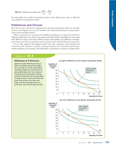
To see this, suppose that Ingrid’s friend Lars also consumes only housing and
restaurant meals. However, Lars has a stronger preference for restaurant meals and a
weaker preference for housing. This difference in preferences is shown in Figure 80.8,

figure 80.8

Differences in Preferences (a) Ingrid’s Preferences and Her Optimal Consumption Bundle

Ingrid and Lars have different preferences, re- Quantity of
flected in the different shapes of their indiffer- restaurant
ence curve maps. So they will choose different meals
Ingrid’s optimal
consumption bundles even when they have the 80 consumption
same possible choices. Each has an income of bundle
70
$2,400 per month and faces prices of $30 per
meal and $150 per room. Panel (a) shows Ingrid’s 60
consumption choice: 8 rooms and 40 restaurant 50
meals. Panel (b) shows Lars’s choice: even I
40 3
though he has the same budget line, he con-
sumes fewer rooms and more restaurant meals. 30 I 2
20
I 1
10
BL
0 2 4 6 8 10 12 14 16
Quantity of rooms
(b) Lars’s Preferences and His Optimal Consumption Bundle
Quantity of
restaurant
meals Lars’s optimal
consumption
80 bundle
70
60
I
50 3
40 I 2
30
20 I 1
10
BL
0 2 4 6 8 10 12 14 16
Quantity of rooms

module 80 Appendix 799