Page 105 - NGTU_paper_withoutVideo

Modern Geomatics Technologies and Applications

COVID-19 prevalence and identify the factors affecting its severe spread. However, there are also gaps in terms of enough
knowledge about the spatial patterns of the disease. [16].
Spatial analysis methods and Geographic Information System (GIS) platforms could provide a wide range of advantages
for practitioners working in this field.

2. Materials and methods

2.1 Data collection
In order to calculate the CIR and CFR values globally, the data of global population, estimation of cumulative total of
COVID-19 incidence rates, and fatality rates (case/100,000 population) were derived. The population data of 2019 for each
country was collected from the World Bank [17]. Besides, COVID-19 cumulative total cases and cumulative total deaths until
January 9, 2021 were obtained from World Health Organization public dashboard [18].
Cumulative incidence rate (CIR) presents the percentage of the number of people who get sick in a given time period [19].
Cumulative fatality rate (CFR) demonstrates the percentage of the number of deaths by a certain disease in a specified period
[20]. After computing the values of CIR and CFR for each country, we entered them into the ArcGIS 10.8 software to continue
analysing the spatial patterns.

2.2 Pattern analysis
Spatial autocorrelation statistics measure a basic property of geographic data-the extent of their interdependence with
data at other locations [21]. Moran’ I is a commonly used indicator of spatial autocorrelation [22], which reveals the tendency
of polygons having similar (linear correlated) values when compared to their neighbours [23]. The value of Moran’s I is
between -1.0 and +1.0, which is an indicator of the spatial pattern. This analysis defined as: (> 0) clustered, (= 0) dispersed,
and (< 0) is random distribution. The spatial distribution of COVID-19 CIRs was obtained by the global Moran’s I according
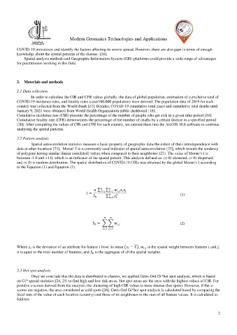
to the Equation (1) and Equation (2).

∑ ∑ =1
=1
,
= (1)
0 ∑ =1 2

= ∑ ∑ (2)
,
0
=1 =1

Where is the deviation of an attribute for feature from its mean ( − ), is the spatial weight between features and ,
,

is equal to the total number of features, and is the aggregate of all the spatial weights.
0

2.3 Hot spot analysis
Once we conclude that the data is distributed in clusters, we applied Getis-Ord Gi*hot spot analysis, which is based
on Gi* spatial statistics [24, 25] to find high and low risk areas. Hot spot areas are the ones with the highest values of CIR. For
positive z-scores derived from the analysis, the clustering of high CIR values is more intense (hot spots). However, if the z-
scores are negative, the area considered as cold spots [26]. Getis-Ord Gi*hot spot analysis is calculated based by comparing the
local sum of the value of each location (country) and those of its neighbours to the sum of all feature values. It is calculated as
follows:

2