Page 258 - Linear Models for the Prediction of Animal Breeding Values 3rd Edition

as another approach to handle censored records in a linear model. In addition, time-
dependent variables could be fitted with an RRM. The records in lactations 1 to 4
were coded as 1 if next lactation was present or 0 otherwise. For censored animals,
current lactations were coded as described but later (future) lactations were regarded
as missing. Thus for uncensored animals, there would be four observations and cen-
sored animals would have a number of observations equal to the current lactation at
which they were censored. In addition to the fixed effects of HYS of calving, quad-
ratic regressions for milk yield and age within herd, and a linear regression for
Holstein percentage, they modelled the survival records of cows fitting a fixed cubic
polynomial for lactation number and orthogonal polynomial of order 3 for additive
animal genetic effects. It is not clear why a permanent environmental effect was not
included in their model. They concluded that RRM could be considered as an alterna-
tive to a proportional hazard model in terms of handling time-dependent variables,
but that the RRM was not very efficient at handling culling towards the end of lacta-
tion 4. This was attributed to lack of adequate data in the last lactation in the study.
The same approach could be used to model survival defined in terms of days or
months of productive life. The details of the methodology of fitting an RRM have
been covered in Chapter 9, therefore only an outline is presented here.
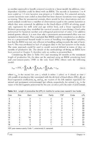
Considering the data in Table 14.1 and assuming 60 months as the maximum
length of productive life, the data can be analysed using an RRM considering herd
and year–season–parity (YSP) as the only fixed (FIX) effects with the following
model:

nf nr nr
i ∑
+
+
y tijk = FIX + f b k ∑ f u jk ∑ f p jk + e tijk (14.1)
jtk
jtk
jtk
k=0 k=0 k=0
where y is the record for cow j, which is either 1 (alive) or 0 (dead) at time t
tijk
(tth month of productive life) associated with the ith level of fixed effects (FIX ); b are
i k
fixed regression coefficients; u and p are vectors of the kth random regression for
jk jk
animal and permanent environmental (pe) effects, respectively, for animal j; f is the
jtk
vector of the kth Legendre polynomial for the cow j at time t; nf is the order of polynomials
Table 14.1. Length of productive life (LPL) in months for some cows reared in two herds.
Cow Sire Dam Herd Parity YSP Code LPL
8 1 2 1 2 3 0 40
9 1 3 1 2 4 1 47
10 4 2 1 1 1 0 22
11 4 9 1 1 2 1 28
12 5 3 1 2 3 1 50
13 5 8 1 1 1 1 33
14 1 6 2 2 4 1 49
15 1 7 2 1 1 1 29
16 5 14 2 1 2 0 23
17 5 6 2 2 3 1 37
18 4 7 2 2 4 0 35
19 4 3 2 1 2 1 30
YSP, year–season–parity. Code: 1, uncensored; 0, censored.

242 Chapter 14