Page 259 - Linear Models for the Prediction of Animal Breeding Values 3rd Edition

fitted as fixed regressions; nr is the order of polynomials for animal and pe effects; and
e is the random residual. Note that for cows 8, 10, 16 and 18, which are censored,
tijk
their records consist of the number of observations equal to their last month alive when
they were censored. Thus cows 8 and 10 have 40 and 22 observations consisting of
ones, respectively. However, for uncensored cows, each has 60 observations consisting
of ones and zeros. Thus cow 9 has a record consisting of 47 ones and 13 zeros. The
model in Eqn 14.1 can be fitted as described in Section 9.3.

14.4.3 Proportional hazard models

In view of the peculiarities associated with survival traits in terms of censoring of
records and the presence of time-dependent covariates (i.e. whose values change with
time), the proportional hazard model has been considered a more appropriate
method of handling survival data. Its wide usage in the analysis of animal breeding
data has been facilitated by the ‘Survival kit’ software by Ducrocq and Solkner
(1998). A new version of the ‘Survival kit’, written in Fortran 90 with an R interface
to make it user friendly, has recently been released (Mészáros et al., 2013). The new
version offers the opportunity to account for the correlated nature of two random
effects, either by specifying a known correlation coefficient or estimating it from the
data. In addition to the computational complexities of the proportional hazard
model, the other disadvantage of the method is the difficulty of applying it in a multi-
trait situation with more than two traits. This is important as most direct measures
of survival traits are obtained late in life; therefore, various traits, mostly linear or
composite type traits such as fore-udder attachment, udder depth, mammary composite
and legs and feet composite, have been used as indirect predictors of survival.
Subsequently in this section, it is assumed that censoring is random, such that the
end time or censoring is independent for all individuals.

Defining some distributions

The basic idea is that survival time follows a distribution (for example, Fig. 14.1) and
the goal is to use data to estimate the parameters of this distribution. Let T be the ran-
dom continuous variable denoting the failure time (death) of an animal, then the survival
function S(t), which is the probability that the animal survives at least until time t, is:
S(t) = Pr(T ³ t) = 1 − Pr(T < t) = 1 − F(t)
where F(t) is the cumulative distribution of T and S(t) can be regarded as the propor-
tion of animals still alive at time t.
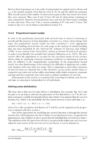
One of the approaches for modelling the survival function is through the hazard
function h(t), which measures the risk of failure of an individual at time t. It specifies the
instantaneous rate of failure at time t, given that the individual has survived up to time t.
The usefulness of the h(t) stems from the fact it can provide the failure rate over time even
when the exact nature of the survival curve is not known. It can be denoted as:

Pr(t £ T < + Dt | t T ³ ) t ft
( )
ht() = lim Dt ®0 =
()
Dt St
Survival Analysis 243