Page 265 - Linear Models for the Prediction of Animal Breeding Values 3rd Edition

Thus given M = [X, Z], where Z is a diagonal matrix considering the cows with records and:
b ⎞
ˆ ⎛
u = ⎜ ⎟
⎝
ˆ a⎠
then vector d = Mu. For instance, if starting values for u in the first iteration were set
to 0.1, then for the first animal, d = m u = 0.30 with m = (1 0 0 0 1 0 1 0 0 0 0 0
1 1 1
0 0 0 0 0 0).
*
Then for animal i, compute r and y and set up the row of equations for ith
ii i
*
animal. For animal 1, r = exp(1*log(40))*exp(0.3) = 53.994 and y = 0 – 53.994
11 1
(1 – 0.3) = −37.760.
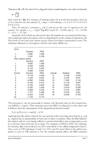
Equation 14.6 is built up and solved after all animals are processed and the itera-
tion continued until convergence. Due to dependencies in the system of equations, the
first levels of herd and year–season–parity effects have been constrained to zero. The
solutions obtained at convergence and the risk ratios (RRS) are:
Herd
Solution RRS
1 0.000 1.000
2 −1.631 0.196
Year–season–parity
Solution RRS
1 0.000 1.000
2 −2.346 0.094
3 −3.149 0.043
4 −2.982 0.051
Animal Solution RRS Animal Solution RRS
1 −0.779 0.459 11 −0.706 0.494
2 −1.233 0.291 12 −0.476 0.621
3 −0.062 0.940 13 −1.902 0.149
4 −0.750 0.472 14 −0.178 0.837
5 −0.758 0.469 15 −0.842 0.431
6 0.238 1.269 16 −0.519 0.595
7 −0.328 0.720 17 −0.115 0.891
8 −1.477 0.228 18 −0.578 0.561
9 −0.533 0.587 19 −0.290 0.748
10 −1.753 0.173

The estimates b can be expressed in relative risk (hazard) ratio by the transforma-
i
tion RRS(b ) = exp(b ). This expression gives the RRS of culling due to that effect and
i i
it follows from the assumption of the proportional hazard model:
h (t; x )/h (t; x ) = exp((x′ − x′ )b)
o a o c a c
implying that the relative hazard for two animals with covariates described by x and
a
x , respectively, is independent of time and of other covariates. Thus the RRS denotes
c
the relative risk of a cow being culled in a certain fixed effect class compared to a cow
in a reference class with risk set to unity. The estimates of RRS in Table 14.1 indicate,
for instance, that cows in herd 2 are 20% more likely to be culled compared to herd 1.
Also, cows in YSP subclasses 2 and 3 are 10% and 4% more likely to be culled com-
pared to cows in YSP subclass 1. For the random animal effect, the RRS estimates

Survival Analysis 249