Page 269 - Linear Models for the Prediction of Animal Breeding Values 3rd Edition

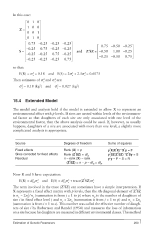
In this case:
é01 0 ù
ê ú
Z = ê 10 0 ú
ê00 1 ú
ê ú
ë 01 0 û
é 075 -0 25. -025. -0 25. ù
.
ê -0..25 - ú é 075. -0 50. -025. ù
.
S = ê -025. 0 75 . 0 25 ú and ZSZ = ê -0 50 1 00 -0 25 ú
′
.
.
.
- ê . 025 - . 0 25 . 075 - . 0 25ú ê ú
ê ú ú ë - ê 025 -0 50 075ú û û
.
.
.
ë - . 025 - . 0 25 - . 025 . 0 75 û
so that:
E(R) = s = 0.18 and E(S) = 2s + 2.5s = 0.6075
2
2
2
e e s
2
Then estimates of s and s are:
2
e s
2
2
s = 0.18 (kg ) and s = 0.027 (kg )
2
2
e s
15.4 Extended Model
The model and analysis hold if the model is extended to allow X to represent an
environmental effect with p levels. If sires are nested within levels of the environmen-
tal factor so that daughters of each sire are only associated with one level of the
environmental factor, then the above analysis could be used. If, however, as usually
happens, daughters of a sire are associated with more than one level, a slightly more
complicated analysis is appropriate.
Source Degrees of freedom Sums of squares
−1
Fixed effects Rank (X) = p y ′ X(X ′ X) X ′ y = F
−1
Sires corrected for fixed effects Rank (Z ′ SZ) = df y ′ SZ(Z ′ SZ) Z ′ Sy = S
S
Residual n – rank (X) – rank y ′ y – F − S = R
(Z ′ SZ) = n – p − df = df
S R
Now R and S have expectation:
2 and 2 2
R
S
e
E(R) = df s e E(S) = df s + trace(Z ′ SZ)s s
The term involved in the trace (Z ′ SZ) can sometimes have a simple interpretation. If
X represents a fixed effect matrix with p levels, then the ith diagonal element of Z ′ SZ
2
is n − Sn /n (summation is from j = 1 to p) where n is the number of daughters of
i. ij .j ij
sire i in fixed effect level j and n = Sn (summation is from j = 1 to p) and n = Sn
.j ij i. ij
(summation is from i = 1 to s). This number was called the effective number of daugh-
ters of sire i by Robertson and Rendel (1954) and measures the loss of information
on a sire because his daughters are measured in different environmental classes. This method
Estimation of Genetic Parameters 253