Page 274 - Linear Models for the Prediction of Animal Breeding Values 3rd Edition

where y = the WWG of the jth calf of the ith sex, p = the effect of the ith sex, a =
ij i j
random effect of the jth calf and e = random error effect.
ijk
In matrix notation, the model is the same as described in Eqn 3.1.
Again, the objective is to illustrate the estimation of variance components s and
2
e
s on a very small example so that the calculations can be expressed concisely.
2
a
In matrix notation, the model is the same as described in Eqn 3.1 with n = 5, p = 2 and
q = 8, with the design matrices as given in Section 3.3. Now y ′ = [2.6, 0.1, 1.0, 3.0, 1.0]
2
2
and, using initial estimates of s = 0.4 and s = 0.2, solutions to MME (Eqn 3.15) are:
e a
Sex effects
Male 2.144
Female 0.602
Animals
1 0.117
2 −0.025
3 −0.222
4 −0.254
5 −0.135
6 0.032
7 0.219
8 −0.305
Then:

(y − Xb − Za) ′ = [0.2022 −0.3661 0.3661 0.6374 −0.8395]
⎡ 0.1884 0.0028 0.0131 0.0878 0.0180 0.0883 0.0554 0.0537⎤
⎢ 0.19668 − ⎥ ⎥
⎢ 0.0028 0.0041 0.0082 0.0949 0.0981 0.0479 0.0443 ⎥
⎢ 0.0131 − 0.0041 0.1826 0.0193 0.0805 0.0090 0.0504 0.0871 ⎥
6
⎢ 0.0878 0.0082 0.0193 0.1711 0.00188 0.0510 0.0971 0.0493 ⎥
2
C s = ⎢ ⎥
22
e
9
⎢ 0.0180 0.0949 0.0805 0.0188 0.1712 0.0679 0.0879 0.0712 ⎥
⎢ 0.0883 0.0981 0.0090 0.0510 0.0679 0.1769 0.0609 0.00877⎥
⎢ ⎥
⎢ 0.0554 0.0479 0.0504 0.0971 0.0879 0.0609 0.1767 0.0672 ⎥
⎣ ⎢ 0.0537 0.0443 0.0871 0.0493 0.0712 0.0877 0.0672 0.1689⎥ ⎦
7
y ′ Py = 4.8193, logdet(V) = −2.6729 and logdet(X ′ V X) = 2.6241 so L = −2.3852
−1
from Eqn 15.1.
Then Eqns 15.2 and 15.3 give:
¶L/¶s = (0.5){(y − Xb − Za) ′ (y − Xb − Za)/s − (n − p − q)/s − trace[C A ]/s }
4
−1
2
2
22
2
e e e a
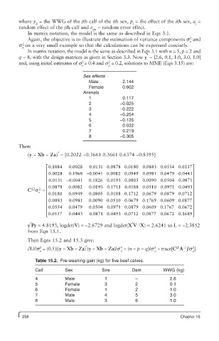
Table 15.2. Pre-weaning gain (kg) for five beef calves.
Calf Sex Sire Dam WWG (kg)
4 Male 1 – 2.6
5 Female 3 2 0.1
6 Female 1 2 1.0
7 Male 4 5 3.0
8 Male 3 6 1.0
258 Chapter 15