Page 278 - Linear Models for the Prediction of Animal Breeding Values 3rd Edition

2
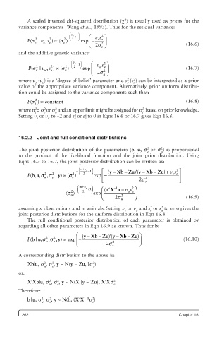
A scaled inverted chi-squared distribution (χ ) is usually used as priors for the
variance components (Wang et al., 1993). Thus for the residual variance:
æ ö
2
- ç v e + 1 ÷ æ vs ö
P(s 2 | v s ) μ (s 2 ) è 2 ø exp - ee ÷
2
ç
,
e e e e ç 2 ÷ (16.6)
è 2s e ø
and the additive genetic variance:
æ v u ö
2
- ç + 1 ÷ æ vs ö
P(s u 2 | v s ) μ (s 2 u ) è 2 ø exp - uu 2 ÷ ÷ (16.7)
2
ç
,
ç
u
u
è 2s u ø
2
2
where v (v ) is a ‘degree of belief’ parameter and s (s ) can be interpreted as a prior
e u e u
value of the appropriate variance component. Alternatively, prior uniform distribu-
tion could be assigned to the variance components such that:
P(s 2 ) μ constant (16.8)
j
2
2
2
where s = s or s and an upper limit might be assigned for s based on prior knowledge.
2
j e u j
2
Setting v or v to −2 and s or s to 0 in Eqns 16.6 or 16.7 gives Eqn 16.8.
2
e u e a
16.2.2 Joint and full conditional distributions
2
2
The joint posterior distribution of the parameters (b, u, s or s ) is proportional
e u
to the product of the likelihood function and the joint prior distribution. Using
Eqns 16.3 to 16.7, the joint posterior distribution can be written as:
⎛ nv e ⎞
+
−
) (y −
−
)
− ⎜ + 1 ⎟ ⎡ (y − Xb Zu ′ Xb Zu) + vs 2 ⎤
⎢
bu 2 , 2 | ) ∝ 2 ) ⎝ 2 ⎠ exp − ee ⎥
y
u
P(, ,ss e (s e 2
⎣ 2s e ⎦
+ ⎞
2
− ⎛ mv u + ⎟ 1 ( ⎛ uA u′ −1 + vs ⎞
⎜
2 ⎝ 2 ⎠ uu
(s u ) exp ⎜ ⎝ ⎝ 2s u 2 ⎟ ⎠ (16.9)
2
2
assuming n observations and m animals. Setting v or v and s or s to zero gives the
e a e a
joint posterior distributions for the uniform distribution in Eqn 16.8.
The full conditional posterior distribution of each parameter is obtained by
regarding all other parameters in Eqn 16.9 as known. Thus for b:
æ (yXb Zu ′ - - )
) (y Xb Zu ö
-
-
ç
bu 2 , 2 , ) y μ exp - ÷ (16.10)
u
P( | ,ss e ç 2 ÷
è 2 s e ø
A corresponding distribution to the above is:
2
2
Xb|u, s , s , y ~ N(y − Zu, Is )
2
u e e
or:
2
X′Xb|u, s , s , y ~ N(X′(y − Zu), X′Xs )
2
2
u e e
Therefore:
ˆ
–1
2
2
2
b|u, s , s , y ~ N(b, (X′X) s )
u e e
262 Chapter 16