Page 283 - Linear Models for the Prediction of Animal Breeding Values 3rd Edition

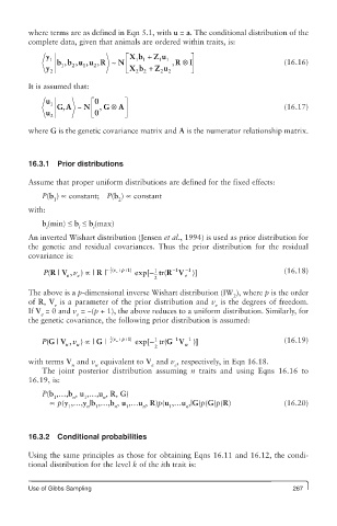
where terms are as defined in Eqn 5.1, with u = a. The conditional distribution of the
complete data, given that animals are ordered within traits, is:
y 1 é Xb + Z u ù
11
11
,
,
,
,
bb uu R ~ N ê , R Ä I ú (16.16)
1
2
1
2
y ë Xb + Z u û
2 2 2 2 2
It is assumed that:
u 1 0 é ù
GA ~ N ê , G Ä A ú (16.17)
,
u 2 ë 0 û
where G is the genetic covariance matrix and A is the numerator relationship matrix.
16.3.1 Prior distributions
Assume that proper uniform distributions are defined for the fixed effects:
P(b ) ∝ constant; P(b ) ∝ constant
1 2
with:
b (min) ≤ b ≤ b (max)
i i i
An inverted Wishart distribution (Jensen et al., 1994) is used as prior distribution for
the genetic and residual covariances. Thus the prior distribution for the residual
covariance is:

-1
1
P( |RV e v , e ) μ | R | - 1 2 ( v e + p+1 ) exp[- tr (R V e -1 )] (16.18)
2
The above is a p-dimensional inverse Wishart distribution (IW ), where p is the order
2
of R, V is a parameter of the prior distribution and v is the degrees of freedom.
e e
If V = 0 and v = −(p + 1), the above reduces to a uniform distribution. Similarly, for
e e
the genetic covariance, the following prior distribution is assumed:
-1
1
P( |GV v , ) μ | G | - 1 2 ( v u + p+1 ) exp[- tr (G V -1 )] (16.19)
u u u
2
with terms V and v equivalent to V and v , respectively, in Eqn 16.18.
u u e e
The joint posterior distribution assuming n traits and using Eqns 16.16 to
16.19, is:
P(b ,…,b , u ,…,u , R, G)
1 n 1 n
∝ p(y ,…,y |b ,…,b , u ,…u , R)p(u ,…u ,|G)p(G)p(R) (16.20)
1 n 1 n 1 n 1 n

16.3.2 Conditional probabilities

Using the same principles as those for obtaining Eqns 16.11 and 16.12, the condi-
tional distribution for the level k of the ith trait is:

Use of Gibbs Sampling 267