Page 282 - Linear Models for the Prediction of Animal Breeding Values 3rd Edition

−1
2
−1
ˆ
u = 0 and (z′ z + A −1 a) s = (3.667) 40 = 10.908
1 1 1 1,1 e
−1
−1
The value of (z′ z + A a) is taken from the diagonal element of the coefficient
1 1 1,1
matrix of the MME for Example 3.1. Assuming the RN from N(0,1) is 0.2067:
1 []
u =+ . . 0 683
0 0 2067 10 98 =
.
1
−1
−1
2
−1
For animal 2, u from Eqn 3.8 = −0.171, and (z′ z + A a) s = (4) 40 = 10.
ˆ
2 1 1 1,1 e
Then from Eqn 16.12, assuming RN from N(0,1) is −1.8025:
1 []
u =- 0 171+ - 1 8025 10 = - 5 871
.
.
.
2
−1
2
−1
−1
Similarly, given that u from Eqn 3.8 = 1.468, (z′ z + A a) s = (4) 40 = 10 and
ˆ
3 1 1 1,1 e
RN = −0.5558, then:
1 []
u = 1 468 0 5558 10 = - 0 290
-
.
.
.
3
−1
−1
−1
ˆ
2
For animal 4, u = 0.0976 from Eqn 3.8, (z′ z + A a) s = (4.667) 40 = 8.571 and
4 1 1 1,1 e
RN = −1.8654, then:
1 []
-
u = 0 0976 1 8654 8 571 = - 5 364
.
.
.
.
4
[1]
[1]
Similar calculations using Eqn 16.12 gave estimates of u , u , u and u to be
[1]
[1]
5 6 7 8
−3.097, −2.577, −1.621 and 0.697, respectively.
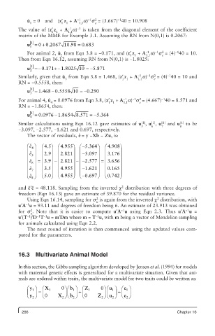
The vector of residuals, eˆ = y −Xb − Zu, is:
ˆ e æ 4 ö æ . 45ö æ 4 955 ö æ -5 364 ö æ 4 908ö
.
.
.
ç ÷ ç ÷ ç ÷ ç ÷ ç ÷
.
.
ç ˆ e 5 ÷ ç . 29 ÷ ÷ ç 2 821 ÷ ç -3.0097 ÷ ç 3 176 ÷
ç
ˆ e ç ÷ = ç . 39 ÷ - ç 2 821 ÷ - - 2 577 ÷ =. ç 3 656 ÷
.
.
ç 6 ÷ ç ÷ ç ÷ ç ÷ ç ÷
1 621
ˆ e ç 7 ÷ ç . 35 ÷ ç 4 955 ÷ ç - . ÷ ç 01655 ÷
.
.
ç ÷ ç ÷ ç ÷ ç ÷ ç ÷
.
0 697
.
è ˆ e 8 ø è . 50 ø è 4 955 ø è - . ø è 0 742 ø
2
ˆ
ˆ
and e′e = 48.118. Sampling from the inverted χ distribution with three degrees of
freedom (Eqn 16.13) gave an estimate of 39.870 for the residual variance.
2
2
Using Eqn 16.14, sampling for s is again from the inverted χ distribution, with
u
−1
u′A u = 93.11 and degrees of freedom being 6. An estimate of 23.913 was obtained
−1
−1
2
for s . Note that it is easier to compute u′A u using Eqn 2.3. Thus u′A u =
u
−1
−1
−1
−1
u′(T )′D T u = m′Dm where m = T u, with m being a vector of Mendelian sampling
for animals calculated using Eqn 2.2.
The next round of iteration is then commenced using the updated values com-
puted for the parameters.
16.3 Multivariate Animal Model
In this section, the Gibbs sampling algorithm developed by Jensen et al. (1994) for models
with maternal genetic effects is generalized for a multivariate situation. Given that ani-
mals are ordered within traits, the multivariate model for two traits could be written as:
æ y ö æ X 1 0 öæ b ö æ Z 1 0 öæ u ö æ e ö
1
+
1
1
+
1 1
ç ÷ = ç ÷ç ÷ ç ÷ç ÷ ç ÷
è y 2 ø è 0 X 2 øè b 2 ø è 0 Z 2 øè u 2 ø è e 2 ø
266 Chapter 16