Page 286 - Linear Models for the Prediction of Animal Breeding Values 3rd Edition

12
11
rhs = rhs + R (y − u ) + R (y − u )
1j 1j 1 1i 2 2i
22
21
rhs = rhs + R (y − u ) + R (y − u )
2j 2j 2 1i 2 2i
Diag = Diag + R
j j
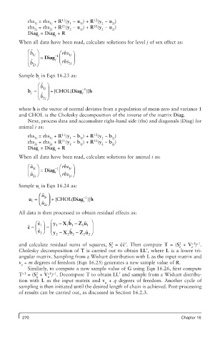
When all data have been read, calculate solutions for level j of sex effect as:
ˆ æ ö
b æ rhs ö
ç j 1 ÷ = Diag - j ç ç j 1 ÷ ÷
1
è b ˆ ç j 2 ø ÷ è rhs j 2 ø
Sample b in Eqn 16.23 as:
j
æ ˆ ö
b
b = ç j 1 ÷ + {CHOL ( Diag )} h
-1
j ÷ j
ç ˆ
b
è 2 j ø
where h is the vector of normal deviates from a population of mean zero and variance 1
and CHOL is the Cholesky decomposition of the inverse of the matrix Diag.
Next, process data and accumulate right-hand side (rhs) and diagonals (Diag) for
animal i as:
12
rhs = rhs + R (y − b ) + R (y − b )
11
1i 1i 1 1j 2 2j
22
rhs = rhs + R (y − b ) + R (y − b )
21
2i 2i 2 1j 2 2j
Diag = Diag + R
i i
When all data have been read, calculate solutions for animal i as:
æ ˆ u ö - 1 æ rhs ö
i 1
i 1
ç ÷ = Diag i ç ÷
è ˆ u i 2 ø è rhs i 2 ø
Sample u in Eqn 16.24 as:
i
⎛ ˆ u 1 i ⎞
u = ⎜ ⎟ + {CHOL (Diag −1 )}h
i
i
⎝ ˆ u i 2 ⎠
All data is then processed to obtain residual effects as:
ˆ
ö æ y - X b - Z ˆ u ö
ˆ e = ç ÷ = ç 1 1 1 1 1 ÷
ˆ e æ 1
ˆ e
ˆ
è 2 ø ç è y - X b - Z 2 ˆ u 2 ÷ ø
2
2
2
2
−1 −1
2
ˆ
ˆ
and calculate residual sums of squares, S = ee′. Then compute T = (S + V ) .
e e e
Cholesky decomposition of T is carried out to obtain LL′, where L is a lower tri-
angular matrix. Sampling from a Wishart distribution with L as the input matrix and
v + m degrees of freedom (Eqn 16.25) generates a new sample value of R.
e
Similarly, to compute a new sample value of G using Eqn 16.26, first compute
−1 −1
−1
2
T = (S + V ) . Decompose T to obtain LL′ and sample from a Wishart distribu-
u u
tion with L as the input matrix and v + q degrees of freedom. Another cycle of
u
sampling is then initiated until the desired length of chain is achieved. Post-processing
of results can be carried out, as discussed in Section 16.2.3.
270 Chapter 16