Page 290 - Linear Models for the Prediction of Animal Breeding Values 3rd Edition

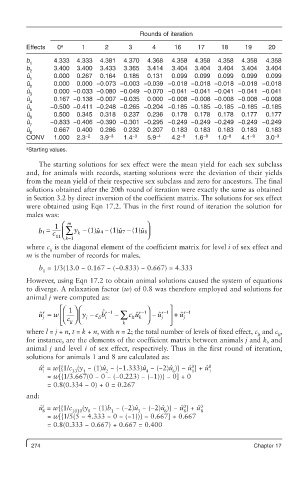
Rounds of iteration
Effects 0 a 1 2 3 4 16 17 18 19 20

b 4.333 4.333 4.381 4.370 4.368 4.358 4.358 4.358 4.358 4.358
1
b 3.400 3.400 3.433 3.365 3.414 3.404 3.404 3.404 3.404 3.404
2
u ˆ 0.000 0.267 0.164 0.185 0.131 0.099 0.099 0.099 0.099 0.099
1
u ˆ 0.000 0.000 −0.073 −0.003 −0.039 −0.018 −0.018 −0.018 −0.018 −0.018
2
u ˆ 0.000 −0.033 −0.080 −0.049 −0.070 −0.041 −0.041 −0.041 −0.041 −0.041
3
u ˆ 0.167 −0.138 −0.007 −0.035 0.000 −0.008 −0.008 −0.008 −0.008 −0.008
4
u ˆ −0.500 −0.411 −0.248 −0.265 −0.204 −0.185 −0.185 −0.185 −0.185 −0.185
5
u ˆ 0.500 0.345 0.318 0.237 0.236 0.178 0.178 0.178 0.177 0.177
6
u ˆ −0.833 −0.406 −0.390 −0.301 −0.295 −0.249 −0.249 −0.249 −0.249 −0.249
7
u ˆ 0.667 0.400 0.286 0.232 0.207 0.183 0.183 0.183 0.183 0.183
8
CONV 1.000 2.3 −2 3.9 −3 1.4 −3 5.9 −4 4.2 −8 1.6 −8 1.0 −8 4.1 −9 3.0 −9
a Starting values.
The starting solutions for sex effect were the mean yield for each sex subclass
and, for animals with records, starting solutions were the deviation of their yields
from the mean yield of their respective sex subclass and zero for ancestors. The final
solutions obtained after the 20th round of iteration were exactly the same as obtained
in Section 3.2 by direct inversion of the coefficient matrix. The solutions for sex effect
were obtained using Eqn 17.2. Thus in the first round of iteration the solution for
males was:
1 ⎛ m ⎞
1 b = c ⎜ ∑ 1 y − (1)u − 7 ˆ (1) 8 u ˆ ⎟ ⎠
4 (1)u −
ˆ
11 ⎝
k
k=
where c is the diagonal element of the coefficient matrix for level i of sex effect and
ii
m is the number of records for males.
b = 1/3(13.0 − 0.167 − (−0.833) − 0.667) = 4.333
1
However, using Eqn 17.2 to obtain animal solutions caused the system of equations
to diverge. A relaxation factor (w) of 0.8 was therefore employed and solutions for
animal j were computed as:
⎛ ⎡ 1 ⎞ ⎛ ⎞ ⎤
r 1−
r
ˆ u = w ⎢ y − cb ˆ r 1− − ∑ c lt k ⎟ − ˆ u r 1− r −1
ˆ u
j ⎥ + ˆ u
j ⎜ c ⎟ ⎜ j li i j
⎣ ⎝ ⎢ ll ⎠ ⎝ k ⎠ ⎦ ⎦ ⎥
where l = j + n, t = k + n, with n = 2; the total number of levels of fixed effect, c and c ,
lt li
for instance, are the elements of the coefficient matrix between animals j and k, and
animal j and level i of sex effect, respectively. Thus in the first round of iteration,
solutions for animals 1 and 8 are calculated as:
1
0
u = w[{1/c (y − (1)uˆ − (−1.333)uˆ − (−2)uˆ )} − uˆ ] + uˆ 0
ˆ
1 33 1 2 4 6 1 1
= w[{1/3.667(0 − 0 − (−0.223) − (−1))} − 0] + 0
= 0.8(0.334 − 0) + 0 = 0.267
and:
0
1
u = w[{1/c (y − (1)b − (−2)u − (−2)u )} − u ] + u ˆ 0
ˆ
ˆ
ˆ
ˆ
8 1010 8 1 3 6 8 8
= w[{1/5(5 − 4.333 − 0 − (−1))} − 0.667] + 0.667
= 0.8(0.333 − 0.667) + 0.667 = 0.400
274 Chapter 17