Page 293 - Linear Models for the Prediction of Animal Breeding Values 3rd Edition

ˆ
ˆ
ˆ
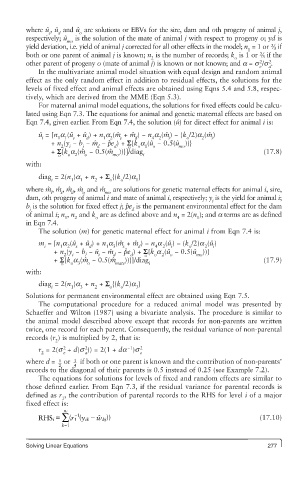
where u , u and u are solutions or EBVs for the sire, dam and oth progeny of animal j,
s d o
respectively; u is the solution of the mate of animal j with respect to progeny o; yd is
ˆ
mo
yield deviation, i.e. yield of animal j corrected for all other effects in the model; n = 1 or ²⁄ if
1 ³
both or one parent of animal j is known; n is the number of records; k is 1 or ²⁄ if the
2 o ³
2
2
other parent of progeny o (mate of animal j) is known or not known; and a = s /s .
e a
In the multivariate animal model situation with equal design and random animal
effect as the only random effect in addition to residual effects, the solutions for the
levels of fixed effect and animal effects are obtained using Eqns 5.4 and 5.8, respec-
tively, which are derived from the MME (Eqn 5.3).
For maternal animal model equations, the solutions for fixed effects could be calcu-
lated using Eqn 7.3. The equations for animal and genetic maternal effects are based on
Eqn 7.4, given earlier. From Eqn 7.4, the solution (u) for direct effect for animal i is:
ˆ
ˆ
u = [n a (uˆ + uˆ ) + n a (mˆ + mˆ ) − n a (mˆ ) − (k /2)a (mˆ )
i 1 1 s d 1 2 s d 4 2 i o 2 i
+ n (y − b − mˆ − p ˆe ) + S{k a (uˆ − 0.5(uˆ ))}
2 i j d d o o 1 o mo
+ S{k a (mˆ − 0.5(mˆ ))}]/diag (17.8)
o o 2 o mo i
with:
diag = 2(n )a + n + S {(k /2)a }
i 1 1 2 o o 1
where m, mˆ , mˆ , mˆ and mˆ are solutions for genetic maternal effects for animal i, sire,
ˆ
i s d o mo
dam, oth progeny of animal i and mate of animal i, respectively; y is the yield for animal i;
i
b is the solution for fixed effect j; p ˆe is the permanent environmental effect for the dam
j d
of animal i; n , n and k are as defined above and n = 2(n ); and a terms are as defined
1 2 o 4 1
in Eqn 7.4.
The solution (m) for genetic maternal effect for animal i from Eqn 7.4 is:
m = [n a (uˆ + uˆ ) + n a (mˆ + mˆ ) − n a (uˆ ) − (k /2)a (uˆ )
i 1 2 s d 1 3 s d 4 2 i o 2 i
+ n (y − b − uˆ − mˆ − p ˆe ) + S{k a (uˆ − 0.5(uˆ ))}
2 i j i d d o o 2 o mo
+ S{k a (mˆ − 0.5(mˆ ))}]/diag (17.9)
o o 3 o mate i
with:
diag = 2(n )a + n + S {(k /2)a }
i 1 3 2 o o 3
Solutions for permanent environmental effect are obtained using Eqn 7.5.
The computational procedure for a reduced animal model was presented by
Schaeffer and Wilton (1987) using a bivariate analysis. The procedure is similar to
the animal model described above except that records for non-parents are written
twice, one record for each parent. Consequently, the residual variance of non-parental
records (r ) is multiplied by 2, that is:
2
2 2 −1 2
2 e a e
r = 2(s + d(s )) = 2(1 + da )s
3
where d = or if both or one parent is known and the contribution of non-parents’
1
2 4
records to the diagonal of their parents is 0.5 instead of 0.25 (see Example 7.2).
The equations for solutions for levels of fixed and random effects are similar to
those defined earlier. From Eqn 7.3, if the residual variance for parental records is
defined as r , the contribution of parental records to the RHS for level i of a major
1
fixed effect is:
RHS ∑ i n ( 1 r − 1 y ( ik − ˆ kj )) (17.10)
i =
w
k 1=
Solving Linear Equations 277