Page 294 - Linear Models for the Prediction of Animal Breeding Values 3rd Edition

ˆ
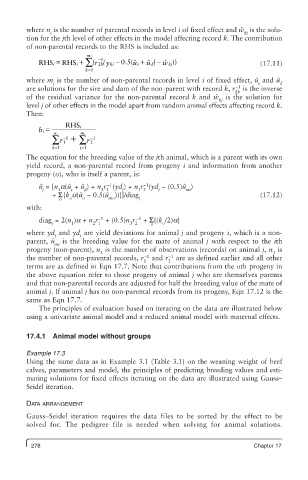
where n is the number of parental records in level i of fixed effect and w is the solu-
i kj
tion for the jth level of other effects in the model affecting record k. The contribution
of non-parental records to the RHS is included as:
m i ˆ
i ∑
−
1
RHS i = RHS + (r 2k ( y − 0.5( s u ˆ + u ˆ d − kj )) (17.11)
) w ˆ
ki
k = 1
where m is the number of non-parental records in level i of fixed effect, uˆ and uˆ
i s d
−1
are solutions for the sire and dam of the non-parent with record k, r is the inverse
2k
of the residual variance for the non-parental record k and w is the solution for
ˆ
kj
level j of other effects in the model apart from random animal effects affecting record k.
Then:
i b = RHS i
ni
∑ r + ∑ r 2 −1
mi
−1
1
k=1 j=1
The equation for the breeding value of the jth animal, which is a parent with its own
yield record, a non-parental record from progeny i and information from another
progeny (o), who is itself a parent, is:
ˆ
−1
−1
u = [n a(uˆ + uˆ ) + n r (yd ) + n r (yd − (0.5)uˆ )
j 1 s d 2 1 j 3 2 i mi
+ S{k a(uˆ − 0.5(uˆ ))}]/diag (17.12)
o o o mo j
with:
−1
−1
diag = 2(n )a + n r + (0.5)n r + S{(k /2)a}
j 1 2 1 3 2 o o
where yd and yd are yield deviations for animal j and progeny i, which is a non-
j i
ˆ
parent, u is the breeding value for the mate of animal j with respect to the ith
mi
progeny (non-parent), n is the number of observations (records) on animal j, n is
2 3
−1
−1
the number of non-parental records, r and r are as defined earlier and all other
1 2
terms are as defined in Eqn 17.7. Note that contributions from the oth progeny in
the above equation refer to those progeny of animal j who are themselves parents
and that non-parental records are adjusted for half the breeding value of the mate of
animal j. If animal j has no non-parental records from its progeny, Eqn 17.12 is the
same as Eqn 17.7.
The principles of evaluation based on iterating on the data are illustrated below
using a univariate animal model and a reduced animal model with maternal effects.
17.4.1 Animal model without groups
Example 17.3
Using the same data as in Example 3.1 (Table 3.1) on the weaning weight of beef
calves, parameters and model, the principles of predicting breeding values and esti-
mating solutions for fixed effects iterating on the data are illustrated using Gauss–
Seidel iteration.
DATA ARRANGEMENT
Gauss–Seidel iteration requires the data files to be sorted by the effect to be
solved for. The pedigree file is needed when solving for animal solutions.

278 Chapter 17