Page 270 - Linear Models for the Prediction of Animal Breeding Values 3rd Edition

of analysis is called Henderson’s method 3 (Henderson, 1953). These methods of
analysis were very popular in that they related to sequential fitting of models and
were relatively easy to compute. One problem is that the terms are generated under
2
a fixed effect model with V = Is and then sums of squares are equated to their
e
expectation under a different variance model. Only in special balanced cases will
2
2
estimation based on R and S lead to efficient estimates of s and s . In general, B is based
s e
2
2
on Z ′ Sy with variance matrix Z ′ SZs + Z ′ SZAZ ′ SZs and these can be transformed
e s
to df independent values Q ′ Z ′ Sy by using arguments similar to those used in Section 6.2
S
on the canonical transformation, where Q is a df n matrix and Q ′ Z ′ SZQ = I and
S
Q ′ Z ′ SZAZ ′ SZQ = W, where W is a diagonal matrix of size df with ith diagonal ele-
S
2
2
ment w . The variance matrix of Q ′ Z ′ Sy is then Is + Ws . Then an analysis of vari-
i e s
ance can be constructed from squaring each of the df elements of Q ′ Z ′ Sy with ith
S
2
sum of squares u with expectation s + w s and R is the residual sum of squares
2
i e i s
2
with expectation E(R) = df s . The individual u are distributed as chi-squared vari-
R e i
2
ables with variance E(u ) . A natural scheme is to fit a linear model in s and s to u
2
2
i s e i
and R. One can also use an iterative scheme with the weight dependent on the esti-
mated parameters.
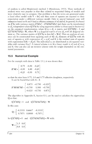
15.5 Numerical Example
For the example with data in Table 15.1, it was shown that:
é 075 - 0 50 - 025ù
.
.
.
ê
′
Z SZ = - 050 1 00 - 025 ú ú
.
.
.
ê
ë - ê 025 - 0 50 075ú û
.
.
.
so that the sires have 0.75, 1.0 and 0.75 effective daughters, respectively.
It can be found that with A = I:
é 0 875 - 0 750 - 0 125ù
.
.
.
ê
′
′
Z SZAZ SZ = - 0 750 1 500 - 0 750 ú ú
.
.
.
ê
.
.
ë - ê 0 125 - 0 750 0.8875ú û
The algorithm in Appendix E, Section E.1, can be used to calculate the eigenvalues
Q so that:
Q ′ Z ′ SZQ = I and Q ′ Z ′ SZAZ ′ SZQ = W
In this case:
- é 0 3333 0 66. . 67 -0 3333. ù
Q = ê ú
.7
ë 0 071 0.0000 -0 707. 1 û
So Q ′ Z ′ SZQ = I and Q ′ Z ′ SZAZ ′ SZQ = W with:
é 1.5 0.0ù
W = ê ú
ë 0.0 1.0 û
254 Chapter 15