Page 329 - Linear Models for the Prediction of Animal Breeding Values 3rd Edition

Thus the solution for b from the MME is equal to the GLS solution for b in Eqn c.3.
ˆ
−1
The proof that aˆ from the MME is equal to GZ′V (y − Xb) in Eqn c.3 was given
ˆ
−1
−1
−1
−1
−1
by Henderson (1963). Replace V in GZ′V (y − Xb) by R – R ZWZ′R , thus:
ˆ
ˆ
−1
−1
−1
−1
GZ′V (y − Xb) = GZ′(R − R ZWZ′R )(y − Xb)
ˆ
−1
−1
−1
= G(Z′R − Z′R ZWZ′R )(y − Xb)
ˆ
−1
−1
= G(I − Z′R ZW)Z′R (y − Xb)
ˆ
−1
−1
−1
= G(W − Z′R Z)WZ′R (y − Xb)
ˆ
−1
−1
−1
= G((Z′RZ + G ) − Z′R Z)WZ′R (y − Xb)
ˆ
−1
−1
−1
= GZ′R Z + I − GZ′R Z)WZ′R (y − Xb)
ˆ
−1
= (I)WZ′R (y − Xb)
ˆ
−1
= WZ′R (y − Xb) = aˆ (See Eqn c.6)
ˆ
ˆ
ˆ
Thus the BLUP of k′b + a = k′b + a, where b and a are solutions to the MME.
ˆ
C.3 Deriving the Equation for Progeny Contribution (PC)
Considering an individual i that has one record with both sire (s) and dam (d) known,
the MME for the three animals can be written (assuming the sire and dam are ances-
tors with unknown parents) as:
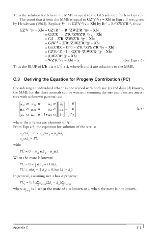
ˆ ⎡
u ⎡ ss a u sd a u si a⎤ ˆ a ⎤ ⎡ 0 ⎤
s
⎢ ⎥ ⎢ ⎥ ⎢ ⎥ (c.8)
⎥ ⎢
⎢ u ds a u dd a u di a ⎥ ⎢ ˆ a = 0 ⎥
d
⎢
⎢ u ⎣ is a u id a 1 + uii a⎥ ˆ a i ⎦ ⎣ ⎥ ⎦
⎦ ⎣
⎥ ⎢1′y
−1
where the u terms are elements of A .
From Eqn c.8, the equation for solution of the sire is:
u aa = 0 − u a a − u aa ˆ
ˆ
ˆ
ss s sd d si i
ˆ
u a a = PC
ss s
with:
PC = 0 − u aaˆ − u aaˆ
sd d si i
When the mate is known:
PC = 0 − 1 aaˆ + (1)aaˆ
2 d i
ˆ
ˆ
ˆ
1
ˆ
PC = a(a − a ) = 0.5a(2a − a )
i 2 d i d
In general, assuming sire s has k progeny:
ˆ
ˆ
PC = 0.5aΣu (2a − a )/Σu
s k prog i m k prog
where u is 1 when the mate of s is known or when the mate is not known.
2
prog 3
Appendix C 313