Page 39 - Linear Models for the Prediction of Animal Breeding Values 3rd Edition

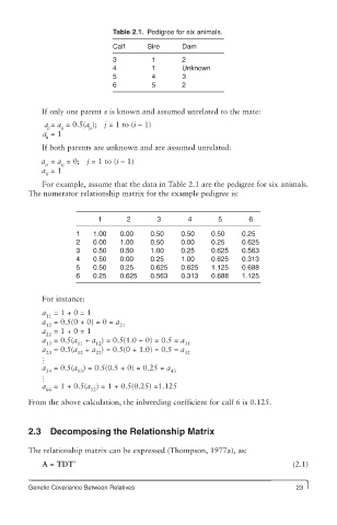
Table 2.1. Pedigree for six animals.
Calf Sire Dam
3 1 2
4 1 Unknown
5 4 3
6 5 2

If only one parent s is known and assumed unrelated to the mate:
a = a = 0.5(a ); j = 1 to (i – 1)
ji ij js
a = 1
ii
If both parents are unknown and are assumed unrelated:
a = a = 0; j = 1 to (i – 1)
ji ij
a = 1
ii
For example, assume that the data in Table 2.1 are the pedigree for six animals.
The numerator relationship matrix for the example pedigree is:

1 2 3 4 5 6

1 1.00 0.00 0.50 0.50 0.50 0.25
2 0.00 1.00 0.50 0.00 0.25 0.625
3 0.50 0.50 1.00 0.25 0.625 0.563
4 0.50 0.00 0.25 1.00 0.625 0.313
5 0.50 0.25 0.625 0.625 1.125 0.688
6 0.25 0.625 0.563 0.313 0.688 1.125

For instance:

a = 1 + 0 = 1
11
a = 0.5(0 + 0) = 0 = a
12 21
a = 1 + 0 = 1
22
a = 0.5(a + a ) = 0.5(1.0 + 0) = 0.5 = a
13 11 12 31
a = 0.5(a + a ) = 0.5(0 + 1.0) = 0.5 = a
23 12 22 32

a = 0.5(a ) = 0.5(0.5 + 0) = 0.25 = a
34 13 43

a = 1 + 0.5(a ) = 1 + 0.5(0.25) =1.125
66 52
From the above calculation, the inbreeding coefficient for calf 6 is 0.125.

2.3 Decomposing the Relationship Matrix

The relationship matrix can be expressed (Thompson, 1977a), as:
A = TDT′ (2.1)

Genetic Covariance Between Relatives 23