Page 41 - Linear Models for the Prediction of Animal Breeding Values 3rd Edition

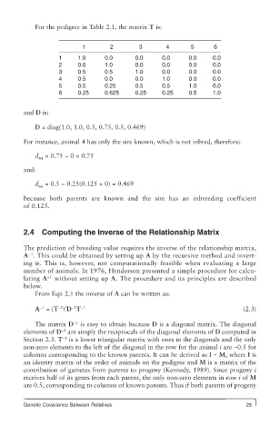
For the pedigree in Table 2.1, the matrix T is:

1 2 3 4 5 6
1 1.0 0.0 0.0 0.0 0.0 0.0
2 0.0 1.0 0.0 0.0 0.0 0.0
3 0.5 0.5 1.0 0.0 0.0 0.0
4 0.5 0.0 0.0 1.0 0.0 0.0
5 0.5 0.25 0.5 0.5 1.0 0.0
6 0.25 0.625 0.25 0.25 0.5 1.0

and D is:

D = diag(1.0, 1.0, 0.5, 0.75, 0.5, 0.469)
For instance, animal 4 has only the sire known, which is not inbred, therefore:

d = 0.75 − 0 = 0.75
44
and:

d = 0.5 − 0.25(0.125 + 0) = 0.469
66
because both parents are known and the sire has an inbreeding coefficient
of 0.125.

2.4 Computing the Inverse of the Relationship Matrix

The prediction of breeding value requires the inverse of the relationship matrix,
−1
A . This could be obtained by setting up A by the recursive method and invert-
ing it. This is, however, not computationally feasible when evaluating a large
number of animals. In 1976, Henderson presented a simple procedure for calcu-
lating A without setting up A. The procedure and its principles are described
−1
below.
From Eqn 2.1 the inverse of A can be written as:

−1
−1
−1
A = (T )′D T −1 (2.3)
−1
The matrix D is easy to obtain because D is a diagonal matrix. The diagonal
−1
elements of D are simply the reciprocals of the diagonal elements of D computed in
−1
Section 2.3. T is a lower triangular matrix with ones in the diagonals and the only
non-zero elements to the left of the diagonal in the row for the animal i are −0.5 for
columns corresponding to the known parents. It can be derived as I − M, where I is
an identity matrix of the order of animals on the pedigree and M is a matrix of the
contribution of gametes from parents to progeny (Kennedy, 1989). Since progeny i
receives half of its genes from each parent, the only non-zero elements in row i of M
are 0.5, corresponding to columns of known parents. Thus if both parents of progeny

Genetic Covariance Between Relatives 25