Page 44 - Linear Models for the Prediction of Animal Breeding Values 3rd Edition

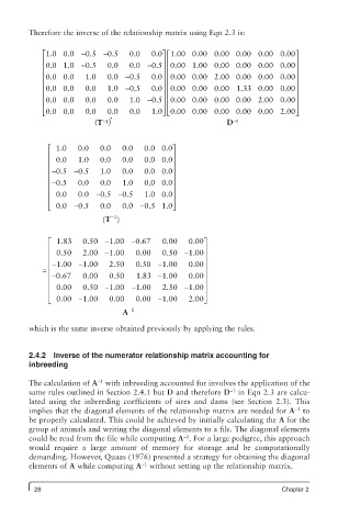
Therefore the inverse of the relationship matrix using Eqn 2.3 is:

⎡ ⎡ 1.0 0.0 − 0.5 − 0.5 0.0 0.0⎤ 1.00 0.00 0.00 0.00 0.00 0.00⎤
⎡ ⎡
⎢ 0.0 1.0 − 0.0 − ⎥ ⎢ ⎥
⎢ 0.5 0.0 0.5 ⎥ ⎢ 0.00 1.000 0.00 0.00 0.00 0.00 ⎥
⎢ 0.0 0.0 1.0 0.0 − 0.5 0.0⎥ 0.00 0.00 2.00 0.00 0.00 0.00⎥
0 ⎢
⎢ ⎥ ⎢ ⎥
3
⎢ 0.0 0.0 0.0 1.0 − 0.5 0.0 ⎥ ⎢ 0.00 0.00 0.00 1.33 0.00 0.00 ⎥
⎢ 0.0 0.0 0.0 0.0 1.0 − 0.5 ⎥ ⎢ 0.00 0.00 0.00 0.00 2.00 0.00 ⎥
⎢ ⎥ ⎢ ⎥
⎦ ⎣ ⎢
⎣ ⎢ 0.0 0.0 0.0 0.0 0.0 1.0⎥ 0.00 0.00 0.00 0.00 0.00 2.00⎥ ⎦
1 ′
(T − ) D −1
⎡ 1.0 0.0 0.0 0.0 0.0 0.0⎤
⎢ ⎥
⎢ 0.0 1.0 0.0 0.0 0.0 0.0 ⎥
⎢ − 0.5 − 0.5 1.0 0.0 0.0 0.0⎥
⎢ ⎥
⎢ −00.5 0.0 0.0 1.0 0.0 0.0 ⎥
⎢ 0.0 0.0 − 0.5 − 0.5 1.0 0.0 ⎥
⎢ ⎥
⎣ ⎢ 0.0 − 0.5 0.0 0.0 − 0.5 1.0⎥ ⎦
0
−1
(T )

é 1.83 0.50 - 1.00 - 0.67 0.00 0.00ù
ê 2.00 - 0.50 - ú ú
ê 0.50 1.00 0.00 1.00 ú
ê - 1.00 - 1.00 2.50 0.50 - 1.00 0.00ú
0
= ê ú
ê - 0.67 0.00 0.50 1.83 - 1.00 0.00 ú
ê 0.00 0.50 -1.00 -1.00 2.50 -1.00 ú
-
ê ú
ë ê 0.00 -1.00 0.00 0.00 -1.00 2.00ú û
A -1

which is the same inverse obtained previously by applying the rules.

2.4.2 Inverse of the numerator relationship matrix accounting for
inbreeding

−1
The calculation of A with inbreeding accounted for involves the application of the
−1
same rules outlined in Section 2.4.1 but D and therefore D in Eqn 2.3 are calcu-
lated using the inbreeding coefficients of sires and dams (see Section 2.3). This
−1
implies that the diagonal elements of the relationship matrix are needed for A to
be properly calculated. This could be achieved by initially calculating the A for the
group of animals and writing the diagonal elements to a file. The diagonal elements
−1
could be read from the file while computing A . For a large pedigree, this approach
would require a large amount of memory for storage and be computationally
demanding. However, Quaas (1976) presented a strategy for obtaining the diagonal
elements of A while computing A without setting up the relationship matrix.
−1

28 Chapter 2