Page 49 - Linear Models for the Prediction of Animal Breeding Values 3rd Edition

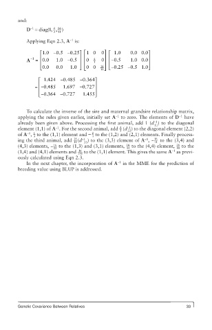
and:
4 16
- 1
D = diag( 1, , )
3 11
−1
Applying Eqn 2.3, A is:
⎡ 1.0 −0.5 −0.25⎤ ⎡ 10 0⎤ ⎡ 1.0 0.0 0.0 ⎤
−1 ⎢ ⎥ ⎢ 4 ⎥ ⎢ − ⎥
A = 0.0 1.0 −0.5 ⎥ ⎢ 0 3 0 ⎥ ⎢ 0.5 1.0 0.0 ⎥
⎢
⎢ ⎣ 0.0 0.0 1.0 ⎥ ⎢ 00 16 ⎥ ⎢ 0.25− − 0.5 1.0 ⎥ ⎦
11⎦ ⎣
6
⎦ ⎣
⎡ 1.424 − 0.485 − 0.364⎤
⎢
= − 0.485 1.697 − 0.727 ⎥ ⎥
⎢
⎢ ⎣ − 0.364 − 0.727 1.455⎥ ⎦ ⎦

To calculate the inverse of the sire and maternal grandsire relationship matrix,
−1
applying the rules given earlier, initially set A to zero. The elements of D have
−1
−1
already been given above. Processing the first animal, add 1 (d ) to the diagonal
11
4
−1
−1
element (1,1) of A . For the second animal, add (d ) to the diagonal element (2,2)
22
3
1
2
−1
of A , to the (1,1) element and − to the (1,2) and (2,1) elements. Finally process-
3
3
16
16
−1
ing the third animal, add (d −1 33 ) to the (3,3) element of A , − to the (3,4) and
11
11
16
(4,3) elements, − to the (1,3) and (3,1) elements, to the (4,4) element, 16 to the
16
22 44 88
−1
16
(1,4) and (4,1) elements and 176 to the (1,1) element. This gives the same A as previ-
ously calculated using Eqn 2.3.
−1
In the next chapter, the incorporation of A in the MME for the prediction of
breeding value using BLUP is addressed.

Genetic Covariance Between Relatives 33