Page 53 - Linear Models for the Prediction of Animal Breeding Values 3rd Edition

BLUP of a under certain assumptions, especially when data span several generations
and may be subject to selection. These assumptions are:
1. Distributions of y, u and e are assumed to be multivariate normal, implying that
traits are determined by many additive genes of infinitesimal effects at many infinitely
unlinked loci (infinitesimal model, see Section 1.2). With the infinitesimal model,
changes in genetic variance resulting from selection, such as gametic disequilibrium
(negative covariance between frequencies of genes at different loci), or from inbreed-
ing and genetic drift, are accounted for in the MME through the inclusion of the
relationship matrix (Sorensen and Kennedy, 1983), as well as assortative mating
(Kemp, 1985).
2. The variances and covariances (R and G) for the base population are assumed to
be known or at least known to proportionality. In practice, variances and covariances
of the base population are never known exactly but, assuming the infinitesimal
model, these can be estimated by restricted (or residual) maximum likelihood
(REML) if data include information on which selection is based.
3. The MME can account for selection if based on a linear function of y (Henderson,
1975) and there is no selection on information not included in the data.
The use of these MME for the prediction of breeding values and estimation of fixed
effects under an animal model is presented in the next section.

3.3 A Model for an Animal Evaluation (Animal Model)

Example 3.1
Consider the data set in Table 3.1 for the pre-weaning gain (WWG) of beef calves
(calves assumed to be reared under the same management conditions).
The objective is to estimate the effects of sex and predict breeding values for all
animals. Assume that s = 20 and s = 40, therefore a = 40 = 2.
2
2
a e 20
The model to describe the observations is:
y = p + a + e
ij i j ij
where: y = the WWG of the jth calf of the ith sex; p = the fixed effect of the ith sex;
ij i
a = random effect of the jth calf; and e = random error effect. In matrix notation the
j ij
model is the same as that described in Eqn 3.1.

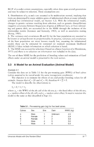
Table 3.1. Pre-weaning gain (kg) for five beef calves.
Calves Sex Sire Dam WWG (kg)
4 Male 1 Unknown 4.5
5 Female 3 2 2.9
6 Female 1 2 3.9
7 Male 4 5 3.5
8 Male 3 6 5.0

Univariate Models with One Random Effect 37