Page 57 - Linear Models for the Prediction of Animal Breeding Values 3rd Edition

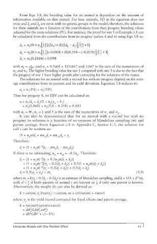
From Eqn 3.8, the breeding value for an animal is dependent on the amount of
information available on that animal. For base animals, YD in the equation does not
ˆ
exist and a and aˆ are zeros with no genetic groups in the model; therefore, the solutions
s d
for these animals are a function of the contributions from their progeny breeding values
adjusted for the mate solutions (PC). For instance, the proof for sire 1 in Example 3.1 can
be calculated from the contributions from its progeny (calves 4 and 6) using Eqn 3.8 as:
() n ()
a +
ˆ a = n 0 + ⎡ 2 ( ˆ )( )( ˆ a − a ˆ )⎤ ( 2 + 1)
2
1 2
1 1 3 ⎣ 3 4 6 2 ⎦ 3
ˆ a = n 0 + ⎡ 2 2 0 018 + ( )( . 0 019 ⎤ )) ( 2 + 1)
)
.
1 0 354 − − (
() n () − (
.
1 1 3 ⎣ 3 ⎦ 3
.
0 2166 =)
ˆ a = n (. 0 0 098
1 3
with n = a and n = 0.5a( + 1)/3.667 and 3.667 is the sum of the numerators of
2
.
1 3 667 3 3
n and n . The higher breeding value for sire 1 compared with sire 3 is due to the fact that
1 3
the progeny of sire 1 have higher proofs after correcting for the solutions of the mates.
The solutions for an animal with a record but with no progeny depend on the aver-
age contributions from its parents and its yield deviation. Equation 3.8 reduces to:
a = n (PA) + n (YD)
i 1 2
Thus for progeny 8, its EBV can be calculated as:
a = n (aˆ + aˆ )/2 + n (y − b )
1 3 6 2 8 1
= n (0.068) + n (5.0 − 4.358) = 0.183
1 2
with n = 2a , n = and 5 is the sum of the numerators of n and n .
1
1
2
2
5
5
1
It can also be demonstrated that for an animal with a record but with no
progeny its solution is a function of an estimate of Mendelian sampling (m) and
parent average. From Equation c.8 in Appendix C, Section C.3, the solution for
calf i can be written as:
(1 + u a)aˆ + au aˆ + au aˆ = y
ii i cs s cd d i
Therefore:
−1
ˆ
a = (1 + u a) [y − au aˆ − au aˆ ]
i ii i is s id d
If there is no inbreeding, u = u = −0.5u . Therefore:
is id ii
−1
ˆ
a = (1 + u a) [y + 0.5u a(aˆ + aˆ )]
i ii i ii s d
−1
= (1 + u a) [(y − 0.5(aˆ + aˆ )) + 0.5(1 + u a)(aˆ + aˆ )]
ii i s d ii s d
−1
= (1 + u a) (y − 0.5(aˆ + aˆ )) + 0.5(aˆ + aˆ )
ii i s d s d
a = 0.5(a + a ) + m (3.9)
ˆ
i s d i
−1
where m = k(y − 0.5aˆ − 0.5aˆ ) is an estimate of Mendelian sampling, and k = 1/(1 + d a),
i i s d
3
1
with d = if both parents of animal i are known or if only one parent is known.
2 4
Alternatively, the weight (k) can also be derived as:
k = cov(m, y )/var(y ) = cov(m, m + e)/(var(m) + var(e))
c c
where y is the yield record corrected for fixed effects and parent average.
c
k = var(m)/(var(m)+var(e))
2
= ds /(ds +s )
2
2
a
a
e
2
= dh /(dh + (1− h ))
2
2
Univariate Models with One Random Effect 41