Page 59 - Linear Models for the Prediction of Animal Breeding Values 3rd Edition

dairy cattle studies aimed at detecting quantitative trait loci using the granddaughter
design (Weller, 2001). The equation for calculating DYD from univariate animal
model evaluations was presented by VanRaden and Wiggans (1991) and its deriva-
tion is briefly outlined here.
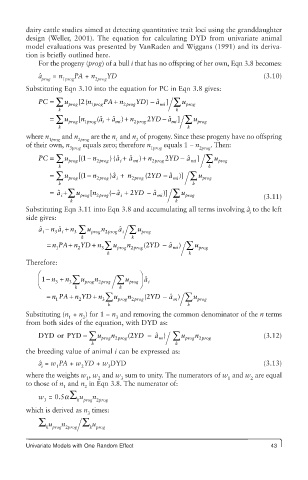
For the progeny (prog) of a bull i that has no offspring of her own, Eqn 3.8 becomes:
a ˆ = n PA + n YD (3.10)
prog 1prog 2prog
Substituting Eqn 3.10 into the equation for PC in Eqn 3.8 gives:
PC = ∑ u prog [( n 1 prog PA + n 2 prog YD) − a ] ∑ u prog
2
ˆ
mi
k k
mi ∑
= ∑ u prog n [ 1 prog (ˆ a + a ˆ ) n 2 prog 2 YD a ˆ ] u prog
−
+
ˆ
i
mi
k k
where n and n are the n and n of progeny. Since these progeny have no offspring
1prog 2prog 1 2
of their own, n equals zero; therefore n equals 1 − n . Then:
3prog 1prog 2prog
PC = ∑ u prog [(1 − n 2 prog ) ( ˆ a + ˆ a ) + n 2 prog 2 YD − ˆ mi ∑ u prog
a ]
mi
i
k k
= ∑ u proog [(1 − n 2 prog )a ˆ i + n 2 prog (2 YD − a ˆ mi )] ∑ u prog
k k
+
= a ˆ i ∑ u prog n [ 2 2prog (− a ˆ i + 2YD − a ˆ mi ∑ u prog
)]
k k (3.11)
Substituting Eqn 3.11 into Eqn 3.8 and accumulating all terms involving a to the left
ˆ
i
side gives:
a ˆ − n 3 a ˆ + n 3 ∑ u prog n 2 prog a ˆ i ∑ u prog
i
i
k k
+
= nPA n YD n ∑ u n (2 YD − a ˆ mi ∑ u
+
)
1 2 3 prog 2 prrog prog
k k
Therefore:
æ ö
ç 1- n 3 + n 3å u prog n 2prog å u prog ÷ a ˆ i
è k k ø
+
+
n
= nPA n YD n 3å u prog 2prog ( 2YD - a ˆ m å u prog
)
2
1
2
k k
Substituting (n + n ) for 1 − n and removing the common denominator of the n terms
1 2 3
from both sides of the equation, with DYD as:
DYD or PYD = å u prog 2 prog 2 ( YD - a ˆ m ) å u prog 2 prog (3.12)
n
n
k k
the breeding value of animal i can be expressed as:
a = w PA + w YD + w DYD (3.13)
ˆ
i 1 2 3
where the weights w , w and w sum to unity. The numerators of w and w are equal
1 2 3 1 2
to those of n and n in Eqn 3.8. The numerator of:
1 2
w = 0.5aΣ u n
3 k prog 2prog
which is derived as n times:
3
Σ u n Σ u
k prog 2prog k prog
Univariate Models with One Random Effect 43