Page 63 - Linear Models for the Prediction of Animal Breeding Values 3rd Edition

The objective is to estimate sex effects and predict breeding values for sires 1, 3 and 4.
2
2
Using the same parameters as in Section 3.3, s = 0.25(20) = 5 and s = 60 − 5 = 55,
s e
therefore a = 55/5 = 11.

SETTING UP THE DESIGN MATRICES AND MME
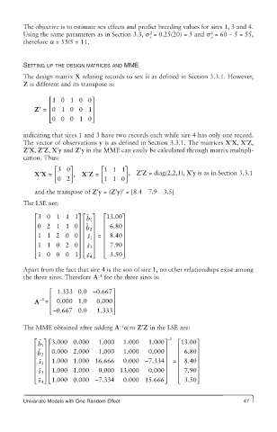
The design matrix X relating records to sex is as defined in Section 3.3.1. However,
Z is different and its transpose is:

⎡10 10 0 ⎤
⎢ ⎥
Z ′ = 0 10 0 1 ⎥
⎢
⎢000 1 0 ⎥ ⎦
⎣
indicating that sires 1 and 3 have two records each while sire 4 has only one record.
The vector of observations y is as defined in Section 3.3.1. The matrices X′X, X′Z,
Z′X, Z′Z, X′y and Z′y in the MME can easily be calculated through matrix multipli-
cation. Thus:
⎡30 ⎤ ⎡1 11 ⎤
′
′
XX = ⎢ ⎥ , XZ = ⎢ ⎥ , Z′Z = diag(2,2,1), X′y is as in Section 3.3.1
⎣ 02 ⎦ ⎣ 11 0 ⎦
and the transpose of Z′y = (Z′y)′ = [8.4 7.9 3.5]
The LSE are:
⎡ 30 1 1 1⎤ ⎡ ˆ ⎤ ⎡13.00 ⎤
1 b
⎢ ⎥ ⎢ ⎢ ⎥ ⎢ ⎥
⎢ 02 1 1 0 ⎥ ˆ 2 b ⎢ ⎥ ⎢ 6.80 ⎥
⎢ 11 2 0 0⎥ ⎢ 1 ˆ s ⎥ = ⎢ 8.40 ⎥
⎢ ⎥ ⎢ ⎥ ⎢ ⎥
⎢ 11 0 2 0 ⎥ ⎢ 3 ˆ s ⎥ ⎢ 7.90 ⎥
⎢ ⎣ 1 0001 ⎥ ⎢ 4 ˆ s ⎦ ⎥ ⎢ ⎣ 3.50 ⎥ ⎦
⎦ ⎣

Apart from the fact that sire 4 is the son of sire 1, no other relationships exist among
−1
the three sires. Therefore A for the three sires is:
⎡ 1.333 0.0 −0.667⎤
−1 ⎢ ⎥
A = ⎢ 0.000 1.0 0.000 ⎥
⎢ ⎣ −0.667 0.0 1.333⎥ ⎦

−1
The MME obtained after adding A a to Z′Z in the LSE are:
ˆ ⎡ 1 b ⎤ ⎡ 3.000 0.000 1.000 1.000 1.000⎤ − 1 ⎡13.00 ⎤
⎢ ⎥ ⎢ ⎥ ⎢ ⎥
ˆ 2 b ⎢ ⎥ ⎢ 0 0.000 2.000 1.000 1.000 0.000 ⎥ ⎢ 6.80 ⎥
⎢ 1 ˆ s ⎥ 1.000 1.000 16.666 0.000 − 7.334⎥ = ⎢ 8.40 ⎥
⎢
⎢ ⎥ ⎢ ⎥ ⎢ ⎥
⎢ 3 ˆ s ⎥ ⎢ 1.000 11.000 0.000 13.000 0.000 ⎥ ⎢ 7.90 ⎥
⎢ 4 ˆ s ⎣ ⎥ ⎢ 1.000 0.000 − 7.334 0.000 15.666 ⎥ ⎦ ⎦ ⎢ ⎣ 3.50 ⎥ ⎦
⎦ ⎣

Univariate Models with One Random Effect 47