Page 66 - Linear Models for the Prediction of Animal Breeding Values 3rd Edition

and:
var(e * ) = var(m ) + var(e )
ijk j ijk
Using Eqn 3.19:

1 2 2
ijk 2 a e
var(e * ) = (1 − F)s + s
In general:
2
j j j a
var(m ) = d (1 − F )s (3.22)
3
1
where d equals or or 1 if both, one or no parents are known, respectively, and F
j 2 4 j
is the average inbreeding for both parents or, if only one parent is known, it is the
inbreeding coefficient of the known parent. F equals zero when no parent is known.
j
Ignoring inbreeding:
2 2 −1 2
e
j
a
j
ijk
var(e * ) = s + d s = (1 + d a )s e
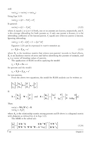
Equation 3.20 can be expressed in matrix notation as:
y = X b + Z a + e * (3.23)
n 1 p
where X is the incidence matrix that relates non-parents’ records to fixed effects,
n
Z is an incidence matrix of zeros and halves identifying the parents of animals, and
1
a is a vector of breeding values of parents.
p
The application of RAM involves applying the model:
y = X b + Za + e
p p
for parents and the model:
y = X b + Z a + e *
n n 1 p
for non-parents.
From the above two equations, the model for RAM analysis can be written as:
y ⎡ ⎤ ⎡ X p⎤ ⎡ Z ⎤ e ⎡ ⎤
⎢ p ⎥ = ⎢ ⎥ b + ⎢ ⎥ p a + ⎢ ⎥
⎣ y ⎢ n⎦ ⎥ ⎣ X n⎦ ⎣ Z 1 ⎦ e ⎣ ⎦
*
If:
⎡ X p⎤ ⎡ Z ⎤ ⎡ R p⎤ ⎡ 2 e 0⎤ ⎡ I ⎤ 0
X = ⎢ ⎥ , W = ⎢ ⎥ and R = ⎢ ⎥ = ⎢ Is ⎥ = ⎢ 1 ⎥ s e 2
2*
*
⎣ X n⎦ ⎣ Z 1⎦ ⎣ R n⎦ ⎣ ⎢ 0 Is ⎦ ⎥ ⎣ 0 + IDa − ⎦
e
Then:
2
var(y) = WA W′s + R
p e
2
p p a
var(a ) = A s
where A is the relationship matrix among parents and D above is a diagonal matrix
p
with elements as defined for d in Eqn 3.22.
j
The MME to be solved are:
′
′
ˆ ⎡ ⎤ ⎡ ′ −1 X R W⎤ −1 ⎡ XR y ⎤
− −1
−1
b XR X
⎢ ⎥ = ⎢ −1 −1 −1 2 ⎥ ⎢ ⎥ (3.24)
′
′
′
−1
ˆ a
⎣ ⎦ ⎣ WR X W R W + A 1/s a ⎦ ⎣ ⎢WR y ⎦ ⎥
50 Chapter 3