Page 65 - Linear Models for the Prediction of Animal Breeding Values 3rd Edition

The similarity of the contributions of calf 8 to the proof of sire 3 in both models
is because it is a non-parent and the contribution is slightly higher under the sire model
due to the lack of adjustment for the breeding value of the mate.

3.5 Reduced Animal Model

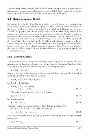
In Section 3.2, the BLUP of breeding value involved setting up equations for
every animal, that is, all parents and progeny. Thus the order of the animal equa-
tions was equal to the number of animals being evaluated. If equations were set
up only for parents, this would greatly reduce the number of equations to be
solved, especially since the number of parents is usually less than the number of
progeny in most data sets. Breeding values of progeny can be obtained by back-
solving from the predicted parental breeding values. Quaas and Pollak (1980)
developed the reduced animal model (RAM), which allowed equations to be set
up only for parents in the MME, and breeding values of progeny are obtained by
back-solving from the predicted parental breeding values. This section presents
the theoretical background for the RAM and illustrates its use for the prediction
of breeding values.

3.5.1 Defining the model

The application of a RAM involves setting up animal equations for parents only and
representing the breeding values of non-parents in terms of parental breeding value.
Thus for the non-parent i, its breeding value can be expressed as:
1
)
a = ( a + a + m i (3.16)
2
i
s
d
where a and a are the breeding values of sire and dam and m is the Mendelian
s d i
sampling. It was shown in Section 2.3 that:
2
i s d a
var(m ) = (0.5 − 0.25(F + F ))s
Let F = (F + F )/2, then:
s d
2
i a
var(m ) = (0.5 − 0.5(F))s
2
a
= 0.5(1 − F)s (3.17)
The animal model applied in Section 3.3 was:
y = p + a + e (3.18)
ijk i j ij
In matrix notation:
y = Xb + Za + e (3.19)
The terms in the above equations have been defined in Section 3.3.
Using Eqn 3.18, Eqn 3.19 can be expressed as:
y = p + a + a + m + e (3.20)
1
1
ijk i 2 s 2 d j ijk
For non-parents, the terms m and e can be combined to form a single residual
j ijk
term e * as:
ijk
e * = m + e (3.21)
ijk j ijk
Univariate Models with One Random Effect 49