Page 54 - Linear Models for the Prediction of Animal Breeding Values 3rd Edition

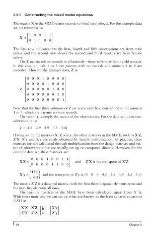
3.3.1 Constructing the mixed model equations

The matrix X in the MME relates records to fixed (sex) effects. For the example data
set, its transpose is:

⎡ 10 0 1 1⎤
X′ = ⎢ ⎥
⎣ 01 1 0 0 ⎦

The first row indicates that the first, fourth and fifth observations are from male
calves and the second row shows the second and third records are from female
calves.
The Z matrix relates records to all animals – those with or without yield records.
In this case, animals 1 to 3 are parents with no records and animals 4 to 8 are
recorded. Thus for the example data, Z is:

⎡ 000 1 0000⎤
⎢ ⎥
⎢ 0000 1 000 ⎥
⎢
Z = 00000 1 0 0⎥
⎢ ⎥
⎢ 000000 1 0 ⎥ ⎥
⎢ ⎣ 0000000 1 ⎥ ⎦

Note that the first three columns of Z are zeros and these correspond to the animals
1 to 3, which are parents without records.
The vector y is simply the vector of the observations. For the data set under con-
sideration, it is:

y′ = [4.5 2.9 3.9 3.5 5.0]
Having set up the matrices X, Z and y, the other matrices in the MME, such as X′Z,
Z′X, X′y and Z′y are easily obtained by matrix multiplication. In practice, these
matrices are not calculated through multiplication from the design matrices and vec-
tor of observations but are usually set up or computed directly. However, for the
example data set, these matrices are:

é 000 1 0 0 1 1ù
¢
¢
¢
XZ = ê ú and Z X is the transpose of XZ
ë 0000 11 00 û
⎛13 0. ⎞
′ =
Xy ⎜ ⎝ 68. ⎟ ⎠ and the transpose of Z′y is (0 0 0 4.5 2.9 3.9 3.5 5.0)
The matrix Z′Z is a diagonal matrix, with the first three diagonal elements zeros and
the next five elements all ones.
−1
The various matrices in the MME have been calculated, apart from A a.
With these matrices, we can set up what are known as the least squares equations
(LSE) as:
′
′ ⎤
′ ⎤ ⎡ ⎤ ˆ
⎡XX XZ b ⎡Xy
⎢ ⎥ ⎢ ⎥ = ⎢ ⎥
′
′
′
⎣ ZX ZZ ⎦ ⎣ ⎦ ⎣ Zy ⎦
a ˆ
38 Chapter 3