Page 212 - Understanding Machine Learning

Multiclass and Ranking
194

That is, (x, y) is composed of k vectors, each of which is of dimension n,where
we set all the vectors to be the all zeros vector except the y’th vector, which is set
to be x. It follows that we can think of w ∈ R nk as being composed of k weight
n
vectors in R ,that is, w = [w 1 ; ... ; w k ], hence the name multivector construction.
By the construction we have that w, (x, y) = w y ,x , and therefore the multiclass
prediction becomes
h(x) = argmax w y ,x .
y∈Y
2
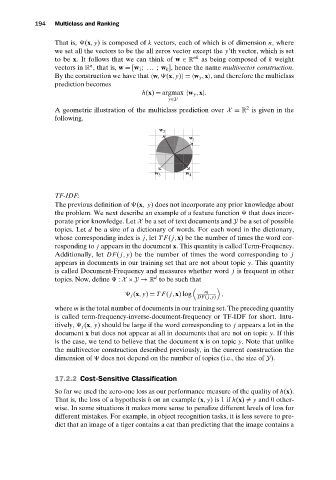
A geometric illustration of the multiclass prediction over X = R is given in the
following.
w 2
w 1

w 3 w 4

TF-IDF:
The previous definition of (x, y) does not incorporate any prior knowledge about
the problem. We next describe an example of a feature function that does incor-
porate prior knowledge. Let X be a set of text documents and Y be a set of possible
topics. Let d be a size of a dictionary of words. For each word in the dictionary,
whose corresponding index is j,let TF( j,x) be the number of times the word cor-
responding to j appears in the document x. This quantity is called Term-Frequency.
Additionally, let DF( j, y) be the number of times the word corresponding to j
appears in documents in our training set that are not about topic y. This quantity
is called Document-Frequency and measures whether word j is frequent in other
d
topics. Now, define : X × Y → R to be such that

j (x, y) = TF( j,x)log m ,
DF( j,y)
where m is the total number of documents in our training set. The preceding quantity
is called term-frequency-inverse-document-frequency or TF-IDF for short. Intu-
itively, j (x, y) should be large if the word corresponding to j appears a lot in the
document x but does not appear at all in documents that are not on topic y.If this
is the case, we tend to believe that the document x is on topic y. Note that unlike
the multivector construction described previously, in the current construction the
dimension of does not depend on the number of topics (i.e., the size of Y).

17.2.2 Cost-Sensitive Classification

So far we used the zero-one loss as our performance measure of the quality of h(x).
That is, the loss of a hypothesis h on an example (x, y)is1 if h(x) = y and 0 other-
wise. In some situations it makes more sense to penalize different levels of loss for
different mistakes. For example, in object recognition tasks, it is less severe to pre-
dict that an image of a tiger contains a cat than predicting that the image contains a