Page 215 - Understanding Machine Learning

17.2 Linear Multiclass Predictors 197

problems. In particular, the RLM technique we have studied in Chapter 13 yields
the multiclass SVM rule:

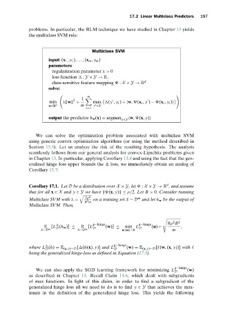
Multiclass SVM

input: (x 1 , y 1 ),...,(x m , y m )
parameters:
regularization parameter λ> 0
loss function : Y × Y → R +
class-sensitive feature mapping : X × Y → R d
solve:
m
1
2

min λ w + max (y , y i ) + w, (x i , y ) − (x i , y i )

w∈R d m y ∈Y
i=1
output the predictor h w (x) = argmax w, (x, y)
y∈Y
We can solve the optimization problem associated with multiclass SVM
using generic convex optimization algorithms (or using the method described in
Section 15.5). Let us analyze the risk of the resulting hypothesis. The analysis
seamlessly follows from our general analysis for convex-Lipschitz problems given
in Chapter 13. In particular, applying Corollary 13.8 and using the fact that the gen-
eralized hinge loss upper bounds the loss, we immediately obtain an analog of
Corollary 15.7:

d
Corollary 17.1. Let D be a distribution over X × Y,let : X × Y → R , and assume
that for all x ∈ X and y ∈ Y we have (x, y) ≤ ρ/2.Let B > 0. Consider running

2ρ 2 m
Multiclass SVM with λ = on a training set S ∼ D and let h w be the output of
2
B m
Multiclass SVM. Then,
*
2
g−hinge g−hinge 8ρ B 2
E [L (h w )] ≤ E [L (w)] ≤ min L (u) + ,
S∼D m D S∼D m D u: u ≤B D m

where L (h) = E (x,y)∼D [ (h(x), y)] and L g−hinge (w) = E (x,y)∼D [ (w,(x, y))] with
D D
being the generalized hinge-loss as defined in Equation (17.3).

g−hinge
We can also apply the SGD learning framework for minimizing L (w)
D
as described in Chapter 14. Recall Claim 14.6, which dealt with subgradients
of max functions. In light of this claim, in order to find a subgradient of the
generalized hinge loss all we need to do is to find y ∈ Y that achieves the max-
imum in the definition of the generalized hinge loss. This yields the following