Page 216 - Understanding Machine Learning

Multiclass and Ranking
198

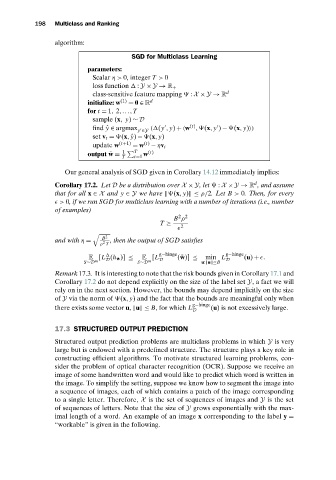
algorithm:
SGD for Multiclass Learning
parameters:
Scalar η> 0, integer T > 0
loss function : Y × Y → R +
class-sensitive feature mapping : X × Y → R d
initialize: w (1) = 0 ∈ R d
for t = 1, 2,...,T
sample (x, y) ∼ D
(t)
( (y , y) + w , (x, y ) − (x, y) )

find ˆy ∈ argmax
y ∈Y
set v t = (x, ˆy) − (x, y)
update w (t+1) = w (t) − ηv t
1 T (t)
output ¯ w = w
T t=1
Our general analysis of SGD given in Corollary 14.12 immediately implies:
d
Corollary 17.2. Let D be a distribution over X × Y,let : X × Y → R , and assume
that for all x ∈ X and y ∈ Y we have (x, y) ≤ ρ/2.Let B > 0. Then, for every

> 0, if we run SGD for multiclass learning with a number of iterations (i.e., number
of examples)
2 2
B ρ
T ≥

2

B 2
and with η = , then the output of SGD satisfies
2
ρ T
g−hinge g−hinge
E [L (h ¯ w )] ≤ E [L ( ¯ w)] ≤ min L (u) +
.
S∼D m D S∼D m D u: u ≤B D
Remark 17.3. It is interesting to note that the risk bounds given in Corollary 17.1 and
Corollary 17.2 do not depend explicitly on the size of the label set Y, a fact we will
rely on in the next section. However, the bounds may depend implicitly on the size
of Y via the norm of (x, y) and the fact that the bounds are meaningful only when
g−hinge
there exists some vector u, u ≤ B,for which L (u) is not excessively large.
D
17.3 STRUCTURED OUTPUT PREDICTION

Structured output prediction problems are multiclass problems in which Y is very
large but is endowed with a predefined structure. The structure plays a key role in
constructing efficient algorithms. To motivate structured learning problems, con-
sider the problem of optical character recognition (OCR). Suppose we receive an
image of some handwritten word and would like to predict which word is written in
the image. To simplify the setting, suppose we know how to segment the image into
a sequence of images, each of which contains a patch of the image corresponding
to a single letter. Therefore, X is the set of sequences of images and Y is the set
of sequences of letters. Note that the size of Y grows exponentially with the max-
imal length of a word. An example of an image x corresponding to the label y =
“workable” is given in the following.