Page 234 - Understanding Machine Learning

Decision Trees
216

Gini Index: Yet another definition of a gain, which is used by the CART
algorithm of Breiman, Friedman, Olshen, and Stone (1984), is the Gini index,

C(a) = 2a(1 − a).

Both the information gain and the Gini index are smooth and concave upper bounds
of the train error. These properties can be advantageous in some situations (see,
for example, Kearns & Mansour (1996)).

18.2.2 Pruning

The ID3 algorithm described previously still suffers from a big problem: The
returned tree will usually be very large. Such trees may have low empirical risk,
but their true risk will tend to be high – both according to our theoretical analysis,
and in practice. One solution is to limit the number of iterations of ID3, leading
to a tree with a bounded number of nodes. Another common solution is to prune
the tree after it is built, hoping to reduce it to a much smaller tree, but still with a
similar empirical error. Theoretically, according to the bound in Equation (18.1), if
we can make n much smaller without increasing L S (h) by much, we are likely to get
a decision tree with a smaller true risk.
Usually, the pruning is performed by a bottom-up walk on the tree. Each node
might be replaced with one of its subtrees or with a leaf, based on some bound or
estimate of L D (h) (for example, the bound in Equation (18.1)). A pseudocode of a
common template is given in the following.

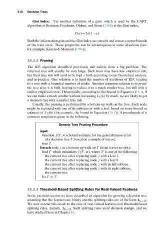
Generic Tree Pruning Procedure

input:
function f (T ,m) (bound/estimate for the generalization error
of a decision tree T , based on a sample of size m),
tree T .
foreach node j in a bottom-up walk on T (from leaves to root):
find T which minimizes f (T ,m), where T is any of the following:

the current tree after replacing node j with a leaf 1.
the current tree after replacing node j with a leaf 0.
the current tree after replacing node j with its left subtree.
the current tree after replacing node j with its right subtree.
the current tree.
let T := T .

18.2.3 Threshold-Based Splitting Rules for Real-Valued Features

In the previous section we have described an algorithm for growing a decision tree
assuming that the features are binary and the splitting rules are of the form 1 [x i =1] .
We now extend this result to the case of real-valued features and threshold-based
splitting rules, namely, 1 [x i <θ] . Such splitting rules yield decision stumps, and we
have studied them in Chapter 10.