Page 238 - Understanding Machine Learning

Nearest Neighbor
220

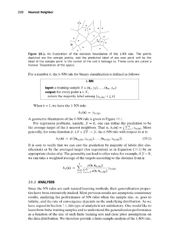
Figure 19.1. An illustration of the decision boundaries of the 1-NN rule. The points
depicted are the sample points, and the predicted label of any new point will be the
label of the sample point in the center of the cell it belongs to. These cells are called a
Voronoi Tessellation of the space.

For a number k,the k-NN rule for binary classification is defined as follows:

k-NN
input: a training sample S = (x 1 , y 1 ),...,(x m , y m )
output: for every point x ∈ X,
return the majority label among {y π i (x) : i ≤ k}

When k = 1, we have the 1-NN rule:
h S (x) = y π 1 (x) .

A geometric illustration of the 1-NN rule is given in Figure 19.1.
For regression problems, namely, Y = R, one can define the prediction to be
1 k
y
the average target of the k nearest neighbors. That is, h S (x) = i=1 π i (x) .More
k
k
generally, for some function φ :(X × Y) → Y,the k-NN rule with respect to φ is:

h S (x) = φ (x π 1 (x) , y π 1 (x) ),...,(x π k (x) , y π k (x) ) . (19.1)
It is easy to verify that we can cast the prediction by majority of labels (for clas-
sification) or by the averaged target (for regression) as in Equation (19.1)by an
appropriate choice of φ. The generality can lead to other rules; for example, if Y = R,
we can take a weighted average of the targets according to the distance from x:
k
ρ(x,x π i (x) )
h S (x) = y π i (x) .
k

i=1 j=1 ρ(x,x π j (x) )
19.2 ANALYSIS
Since the NN rules are such natural learning methods, their generalization proper-
ties have been extensively studied. Most previous results are asymptotic consistency
results, analyzing the performance of NN rules when the sample size, m,goes to
infinity, and the rate of convergence depends on the underlying distribution. As we
have argued in Section 7.4, this type of analysis is not satisfactory. One would like to
learn from finite training samples and to understand the generalization performance
as a function of the size of such finite training sets and clear prior assumptions on
the data distribution. We therefore provide a finite-sample analysis of the 1-NN rule,