Page 240 - Understanding Machine Learning

Nearest Neighbor
222

y ∼ η(x)and y π 1 (x) ∼ η(π 1 (x)). It follows that
E[L D (h S )] = E [1 [y =y ] ]

m
S S x ∼D ,x∼D X ,y∼η(x),y ∼η(π 1 (x))

X

= E P [y = y ] . (19.2)
m

S x ∼D ,x∼D X y∼η(x),y ∼η(π 1 (x))
X
We next upper bound P y∼η(x),y ∼η(x ) [y = y ] for any two domain points x,x :

P [y = y ] = η(x )(1 − η(x)) + (1 − η(x ))η(x)

y∼η(x),y ∼η(x )
= (η(x) − η(x) + η(x ))(1 − η(x))

+ (1 − η(x) + η(x) − η(x ))η(x)
= 2η(x)(1 − η(x)) + (η(x) − η(x ))(2η(x) − 1).

Using |2η(x) − 1|≤ 1 and the assumption that η is c-Lipschitz, we obtain that the
probability is at most:

P [y = y ] ≤ 2η(x)(1 − η(x)) + c x − x .

y∼η(x),y ∼η(x )

Plugging this into Equation (19.2) we conclude that
E[L D (h S )] ≤ E[2η(x)(1 − η(x))] + c E [ x − x π 1 (x) ].
S x S,x
Finally, the error of the Bayes optimal classifier is

L D (h ) = E[min{η(x),1 − η(x)}] ≥ E[η(x)(1 − η(x))].
x x
Combining the preceding two inequalities concludes our proof.
The next step is to bound the expected distance between a random x and its
closest element in S. We first need the following general probability lemma. The
lemma bounds the probability weight of subsets that are not hit by a random sample,
as a function of the size of that sample.
Lemma 19.2. Let C 1 ,...,C r be a collection of subsets of some domain set, X.Let S
be a sequence of m points sampled i.i.d. according to some probability distribution, D
over X. Then,
 
r
E  P[C i ]  ≤ .
m me
S∼D
i:C i ∩S=∅
Proof. From the linearity of expectation, we can rewrite:
 
r

E  P[C i ]  = P[C i ]E 1 [C i ∩S=∅] .
S S
i:C i ∩S=∅ i=1
Next, for each i we have
m −P[C i ]m
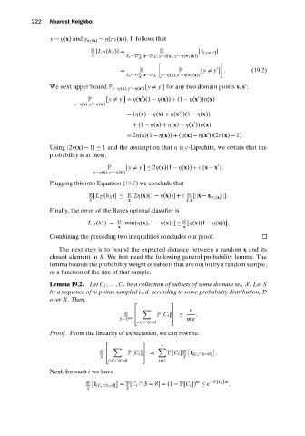
E 1 [C i ∩S=∅] = P[C i ∩ S =∅] = (1 − P[C i ]) ≤ e .
S S