Page 179 - Data Science Algorithms in a Week

Time Series Analysis

2. Electronics shop's sales. Using the data in the electronics shop's sales example,
predict the sales for every month of the year 2019.

Analysis:

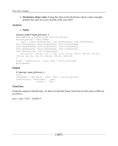
1. Input:

source_code/7/year_bitcoin.r
#Determining a linear trend line for Bitcoin
bitcoin_prices = data.frame(
year = c(2010.91666666666, 2011.41666666666, 2011.91666666666,
2012.41666666666, 2012.91666666666, 2013.41666666666,
2013.91666666666, 2014.41666666666, 2014.91666666666,
2015.41666666666, 2015.91666666666, 2016.41666666666,
2016.91666666666, 2017.41666666666),
btc_price = c(0.23, 9.57, 3.06, 5.27, 12.56, 129.3, 946.92, 629.02,
378.64, 223.31, 362.73, 536.42, 753.25, 2452.18)
)
model = lm(btc_price ~ year, data = bitcoin_prices)
print(model)
Output:

$ Rscript year_bitcoin.r
Call:
lm(formula = btc_price ~ year, data = bitcoin_prices)
Coefficients: (Intercept) year
-431962.9 214.7
Trend line:

From the output of the Rscript, we find out that the linear trend line for the price of Bitcoin
in USD is:
price = year * 214.7 - 431962.9

[ 167 ]