Page 24 - Libro vascular I

ULTRASOUND AND IMAGING 15
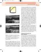
Input signal
A: An example of a compression curve, showing how the amplitude of the signal to be displayed
relates to the amplitude of the input signal. This compression curve accentuates the differences in the lower to mid-range amplitude signal. B and C show the same carotid plaque imaged using two different compression curves.
lowest or the highest signals present or by com- pressing the signal. The signal can be compressed using a nonlinear amplifier. This applies more gain to lower amplitude signals than higher amplitude signals, so reducing the dynamic range of the signal to be displayed. Figure 2.12A gives an example of a compression curve, showing how the amplitude
of the signal to be displayed relates to the amplitude of the input signal. The input signal is the received signal, which has already been amplified by the TGC. This compression curve accentuates the dif- ferences in lower to mid-range amplitude signals. The choice of compression curve used depends on what aspect of the image is important in a given application—for example, the fine detail of back- scatter from tissue or the presence of large bound- aries, such as vessel walls. There are usually a range of compression curves available on modern scan- ners, which are often selected automatically by the system, depending on the selected application (e.g., vascular or abdominal). Figure 2.12B and C shows the same carotid plaque imaged using two different compression curves. The dynamic range of signals arriving at the transducer that can be displayed is defined as the ratio of the largest echo amplitude that does not cause saturation, resulting in peak white, to the smallest echo that can be differenti- ated from noise. Some modern scanners claim to have a dynamic range of 150 dB.
Finally, the scanner uses a gray-scale map to assign a level of gray dependent on the amplitude of amplified signal, to produce the gray-scale image. Some systems have a choice of gray-scale maps, used in different applications, and these will affect the appearance of the image. It is helpful for the sonog- rapher to refer to the scanner operator manual and to explore the effect of the compression curves and gray-scale maps used on the image obtained.
TRANSDUCER DESIGNS AND
BEAM FORMING
In order to produce a two-dimensional (2D) image, the ultrasound beam has to pass through adjacent areas of the tissue. This can be done by physically moving the transducer, and in early real-time scan- ners this was performed by rocking or rotating the transducer element. Many modern electronic imaging transducers are typically made up of 128 elements arranged in a row (Fig. 2.13A), often about 4 cm long. These are known as linear array transducers. If a group of elements are all excited simultaneously (Fig. 2.14A), the wavelets will interfere to produce a beam that is perpendicular to the transducer face. The groups of elements within the array that are excited can be varied to
A
B
C
Figure 2.12
Chap-02.qxd 29~8~04 13:20 Page 15
Displayed signal