Page 59 - Basic _ Clinical Pharmacology ( PDFDrive )

CHAPTER 3 Pharmacokinetics & Pharmacodynamics: Rational Dosing & the Time Course of Drug Action 45

TABLE 3–2 Physical volumes (in L/kg body weight)
of some body compartments into which
drugs may be distributed.
A Compartment
Concentration and Volume Examples of Drugs

Water
Total body water Small water-soluble molecules: eg, ethanol
1
Blood 0 Time (0.6 L/kg )
Extracellular water Larger water-soluble molecules: eg,
(0.2 L/kg) gentamicin
Plasma (0.04 L/kg) Large protein molecules: eg, antibodies
B Fat (0.2-0.35 L/kg) Highly lipid-soluble molecules: eg,
Concentration Bone (0.07 L/kg) Certain ions: eg, lead, fluoride
diazepam

1
An average figure. Total body water in a young lean person might be 0.7 L/kg; in an
obese person, 0.5 L/kg.
Blood 0 Time

Added together, these separate clearances equal total systemic
clearance:
C (3a)
Concentration

(3b)
Extravascular Blood 0 Time
volume
(3c)

(3d)
D “Other” tissues of elimination could include the lungs and
Concentration additional sites of metabolism, eg, blood or muscle.

The two major sites of drug elimination are the kidneys and
the liver. Clearance of unchanged drug in the urine represents
Extravascular Blood 0 Time renal clearance. Within the liver, drug elimination occurs via
volume
biotransformation of parent drug to one or more metabolites, or
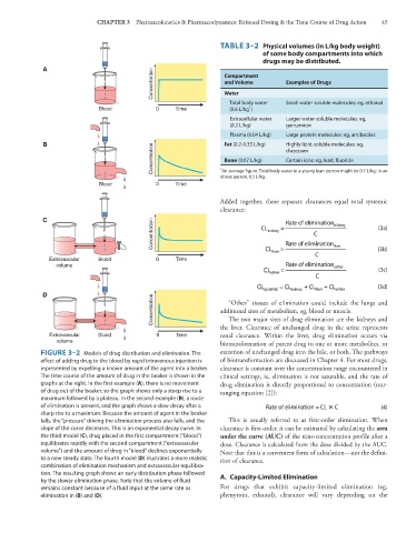
FIGURE 3–2 Models of drug distribution and elimination. The excretion of unchanged drug into the bile, or both. The pathways
effect of adding drug to the blood by rapid intravenous injection is of biotransformation are discussed in Chapter 4. For most drugs,
represented by expelling a known amount of the agent into a beaker. clearance is constant over the concentration range encountered in
The time course of the amount of drug in the beaker is shown in the clinical settings, ie, elimination is not saturable, and the rate of
graphs at the right. In the first example (A), there is no movement drug elimination is directly proportional to concentration (rear-
of drug out of the beaker, so the graph shows only a steep rise to a ranging equation [2]):
maximum followed by a plateau. In the second example (B), a route
of elimination is present, and the graph shows a slow decay after a (4)
sharp rise to a maximum. Because the amount of agent in the beaker
falls, the “pressure” driving the elimination process also falls, and the This is usually referred to as first-order elimination. When
slope of the curve decreases. This is an exponential decay curve. In clearance is first-order, it can be estimated by calculating the area
the third model (C), drug placed in the first compartment (“blood”) under the curve (AUC) of the time-concentration profile after a
equilibrates rapidly with the second compartment (“extravascular dose. Clearance is calculated from the dose divided by the AUC.
volume”) and the amount of drug in “blood” declines exponentially Note that this is a convenient form of calculation—not the defini-
to a new steady state. The fourth model (D) illustrates a more realistic tion of clearance.
combination of elimination mechanism and extravascular equilibra-
tion. The resulting graph shows an early distribution phase followed A. Capacity-Limited Elimination
by the slower elimination phase. Note that the volume of fluid
remains constant because of a fluid input at the same rate as For drugs that exhibit capacity-limited elimination (eg,
elimination in (B) and (D). phenytoin, ethanol), clearance will vary depending on the