Page 57 - Microeconomics, Fourth Edition

c02demandandsupplyanalysis.qxd 7/14/10 11:09 AM Page 31

2.1 DEMAND, SUPPLY, AND MARKET EQUILIBRIUM 31
interpretation of the demand curve that we will return to in later chapters. The demand
curve tells us the highest price that the “market will bear” for a given quantity or sup-
ply of output. Thus, in Figure 2.2, if suppliers of corn offered, in total, 14 billion
bushels for sale, the highest price that the corn would fetch would be $3 per bushel.
Other factors besides price affect the quantity of a good demanded. The prices of
related goods, consumer incomes, consumer tastes, and advertising are among the fac-
tors that we expect would influence the demand for a typical product. However, the
demand curve focuses only on the relationship between the price of the good and the
quantity of the good demanded. When we draw the demand curve, we imagine that
all other factors that affect the quantity demanded are fixed.
The demand curve in Figure 2.2 slopes downward, indicating that the lower the
price of corn, the greater the quantity of corn demanded, and the higher the price of
corn, the smaller the quantity demanded. The inverse relationship between price and
quantity demanded, holding all other factors that influence demand fixed, is called the law law of demand The
of demand. Countless studies of market demand curves confirm the inverse relation- inverse relationship between
ship between price and quantity demanded, which is why we call the relationship a the price of a good and the
law. Still, you might wonder about so-called luxury goods, such as perfume, designer quantity demanded, when
labels, or crystal. It is alleged that some consumers purchase more of these goods all other factors that influ-
ence demand are held
2
at higher prices because a high price indicates superior quality. However, these ex- fixed.
amples do not violate the law of demand because all of the other factors influencing
demand for these goods are not held fixed while the price changes. Consumers’ percep-
tions of the quality of these goods have also changed. If consumers’ perceptions of
quality could be held constant, then we would expect that consumers would purchase
less of these luxury goods as the price goes up.

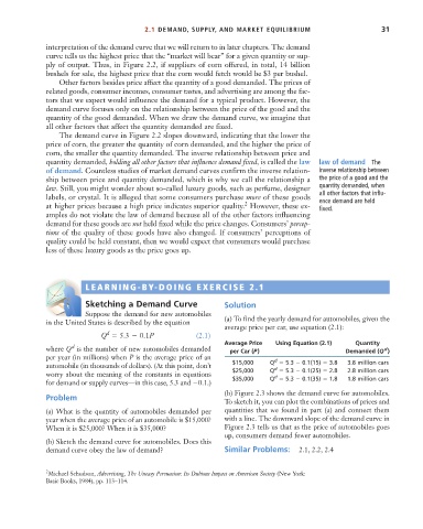
LEARNING-BY-DOING EXERCISE 2.1
S
E D
Sketching a Demand Curve Solution
Suppose the demand for new automobiles
in the United States is described by the equation (a) To find the yearly demand for automobiles, given the
average price per car, use equation (2.1):
d
Q 5.3 0.1P (2.1)
Average Price Using Equation (2.1) Quantity
d
where Q is the number of new automobiles demanded per Car (P) Demanded (Q )
d
per year (in millions) when P is the average price of an d
automobile (in thousands of dollars). (At this point, don’t $15,000 Q 5.3 0.1(15) 3.8 3.8 million cars
d
worry about the meaning of the constants in equations $25,000 Q 5.3 0.1(25) 2.8 2.8 million cars
d
$35,000
Q 5.3 0.1(35) 1.8
1.8 million cars
for demand or supply curves––in this case, 5.3 and 0.1.)
(b) Figure 2.3 shows the demand curve for automobiles.
Problem
To sketch it, you can plot the combinations of prices and
(a) What is the quantity of automobiles demanded per quantities that we found in part (a) and connect them
year when the average price of an automobile is $15,000? with a line. The downward slope of the demand curve in
When it is $25,000? When it is $35,000? Figure 2.3 tells us that as the price of automobiles goes
up, consumers demand fewer automobiles.
(b) Sketch the demand curve for automobiles. Does this
demand curve obey the law of demand? Similar Problems: 2.1, 2.2, 2.4
2 Michael Schudson, Advertising, The Uneasy Persuasion: Its Dubious Impact on American Society (New York:
Basic Books, 1984), pp. 113–114.