Page 61 - Microeconomics, Fourth Edition

c02demandandsupplyanalysis.qxd 6/14/10 1:39 PM Page 35

2.1 DEMAND, SUPPLY, AND MARKET EQUILIBRIUM 35
which implies P 100. Thus, the equilibrium price is Thus, the equilibrium quantity is 100,000 barrels per
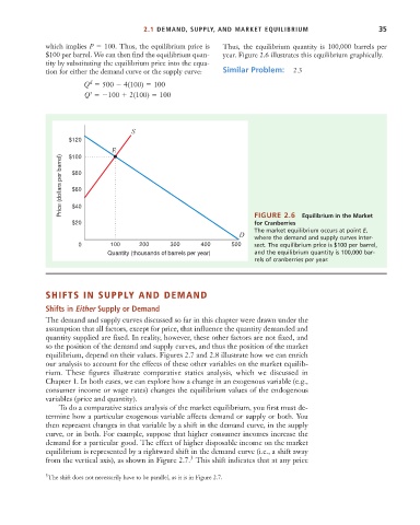
$100 per barrel. We can then find the equilibrium quan- year. Figure 2.6 illustrates this equilibrium graphically.
tity by substituting the equilibrium price into the equa-
tion for either the demand curve or the supply curve: Similar Problem: 2.3
d
Q 500 4(100) 100
s
Q 100 2(100) 100

S
$120
E
$100
Price (dollars per barrel) $80

$60

$40

for Cranberries
$20 FIGURE 2.6 Equilibrium in the Market
The market equilibrium occurs at point E,
D
where the demand and supply curves inter-
0 100 200 300 400 500 sect. The equilibrium price is $100 per barrel,
Quantity (thousands of barrels per year) and the equilibrium quantity is 100,000 bar-
rels of cranberries per year.

SHIFTS IN SUPPLY AND DEMAND
Shifts in Either Supply or Demand
The demand and supply curves discussed so far in this chapter were drawn under the
assumption that all factors, except for price, that influence the quantity demanded and
quantity supplied are fixed. In reality, however, these other factors are not fixed, and
so the position of the demand and supply curves, and thus the position of the market
equilibrium, depend on their values. Figures 2.7 and 2.8 illustrate how we can enrich
our analysis to account for the effects of these other variables on the market equilib-
rium. These figures illustrate comparative statics analysis, which we discussed in
Chapter 1. In both cases, we can explore how a change in an exogenous variable (e.g.,
consumer income or wage rates) changes the equilibrium values of the endogenous
variables (price and quantity).
To do a comparative statics analysis of the market equilibrium, you first must de-
termine how a particular exogenous variable affects demand or supply or both. You
then represent changes in that variable by a shift in the demand curve, in the supply
curve, or in both. For example, suppose that higher consumer incomes increase the
demand for a particular good. The effect of higher disposable income on the market
equilibrium is represented by a rightward shift in the demand curve (i.e., a shift away
3
from the vertical axis), as shown in Figure 2.7. This shift indicates that at any price
3 The shift does not necessarily have to be parallel, as it is in Figure 2.7.