Page 720 - Microeconomics, Fourth Edition

c16GeneralEquilibriumTheory.qxd 8/16/10 9:14 PM Page 694

694 CHAPTER 16 GENERAL EQUILIBRIUM THEORY
DERIVING THE MARKET DEMAND CURVES
FOR LABOR AND CAPITAL

Given the production function for a typical energy producer, the marginal products
of labor and capital are

1 1 2 2 1 2
3 1
3 1
MP a b1.89l k l , and MP a b1.89l k k
3
3
l
k
3 3
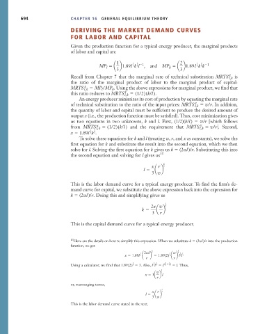
Recall from Chapter 7 that the marginal rate of technical substitution MRTS x l, k is
the ratio of the marginal product of labor to the marginal product of capital:
x
MRTS l, k MP /MP . Using the above expressions for marginal product, we find that
k
l
this ratio reduces to MRTS x l, k (1/2)(k/l ).
An energy producer minimizes its cost of production by equating the marginal rate
x
of technical substitution to the ratio of the input prices: MRTS l, k w/r. In addition,
the quantity of labor and capital must be sufficient to produce the desired amount of
output x (i.e., the production function must be satisfied). Thus, cost minimization gives
us two equations in two unknowns, k and l. First, (1/2)(k/l ) w/r [which follows
x
x
from MRTS l, k (1/2)(k/l ) and the requirement that MRTS l, k w/r . Second,
1 2
x 1.89l k .
3
3
To solve these equations for k and l (treating w, r, and x as constants), we solve the
first equation for k and substitute the result into the second equation, which we then
solve for l. Solving the first equation for k gives us k (2wl )/r. Substituting this into
the second equation and solving for l gives us 13
2
x r 3
l a b
3 w
This is the labor demand curve for a typical energy producer. To find the firm’s de-
mand curve for capital, we substitute the above expression back into the expression for
k (2wl )/r. Doing this and simplifying gives us
1
2x w 3
k a b
3 r
This is the capital demand curve for a typical energy producer.

13 Here are the details on how to simplify this expression. When we substitute k (2wl)/r into the production
function, we get
2 2
1 2wl 3 2 w 3 2 1

x 1.89l 3 a b 1.89(2) 3 a b l 3 l 3
r r
2 2 1 ( 2 1
Using a calculator, we find that 1.89(2) 3 3. Also, l 3 l 3 l 3 3 ) l. Thus,

2
w 3
x 3a b l
r
or, rearranging terms,
2
x r 3
l a b
3 w
This is the labor demand curve stated in the text.