Page 732 - Microeconomics, Fourth Edition

c17ExternalitiesandPublicGoods.qxd 8/22/10 4:56 AM Page 706

706 CHAPTER 17 EXTERNALITIES AND PUBLIC GOODS

s
Optimal emissions fee = P* – P

A
MSC
MPC + Tax = Market supply + Tax
Price P* MPC = Market supply
B
G K
1
P
E H N
s
P
R
F D
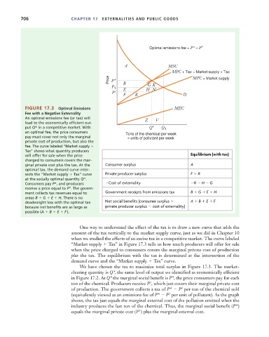
FIGURE 17.3 Optimal Emissions MEC
Fee with a Negative Externality
An optimal emissions fee (or tax) will
lead to the economically efficient out- Z V
put Q* in a competitive market. With Q* Q 1
an optimal fee, the price consumers Tons of the chemical per week
pay must cover not only the marginal = units of pollutant per week
private cost of production, but also the
fee. The curve labeled “Market supply
Tax” shows what quantity producers
will offer for sale when the price Equilibrium (with tax)
charged to consumers covers the mar-
ginal private cost plus the tax. At the Consumer surplus A
optimal tax, the demand curve inter-
sects the “Market supply Tax” curve Private producer surplus F R
at the socially optimal quantity Q*.
Consumers pay P*, and producers Cost of externality R H G
s
receive a price equal to P . The govern-
ment collects tax revenues equal to Government receipts from emissions tax B G E H
areas B G E H. There is no
deadweight loss with the optimal tax Net social benefits (consumer surplus A B E F
because net benefits are as large as private producer surplus cost of externality)
possible (A B E F ).

One way to understand the effect of the tax is to draw a new curve that adds the
amount of the tax vertically to the market supply curve, just as we did in Chapter 10
when we studied the effects of an excise tax in a competitive market. The curve labeled
“Market supply Tax” in Figure 17.3 tells us how much producers will offer for sale
when the price charged to consumers covers the marginal private cost of production
plus the tax. The equilibrium with the tax is determined at the intersection of the
demand curve and the “Market supply Tax” curve.
We have chosen the tax to maximize total surplus in Figure 17.3. The market-
clearing quantity is Q*, the same level of output we identified as economically efficient
in Figure 17.2. At Q* the marginal social benefit is P*, the price consumers pay for each
s
ton of the chemical. Producers receive P , which just covers their marginal private cost
s
of production. The government collects a tax of P* P per ton of the chemical sold
s
(equivalently viewed as an emissions fee of P* P per unit of pollutant). As the graph
shows, the tax just equals the marginal external cost of the pollution emitted when the
industry produces the last ton of the chemical. Thus, the marginal social benefit (P*)
s
equals the marginal private cost (P ) plus the marginal external cost.