Page 736 - Microeconomics, Fourth Edition

c17ExternalitiesandPublicGoods.qxd 8/22/10 4:56 AM Page 710

710 CHAPTER 17 EXTERNALITIES AND PUBLIC GOODS

MSC = MPC + MEC

Price of driving $8.00 G MPC (supply)

B MEC
5.75
A
Optimal peak
5.00
toll = $1.75
4.00 Peak demand
Optimal off- M E (marginal benefit)
peak toll 2.50 T
$0.50 2.00 I
Off-peak demand
N L
(marginal benefit)
U
0
2
Q 1 Q Q 3 Q 4 Q 5
Traffic volume (vehicles per hour)
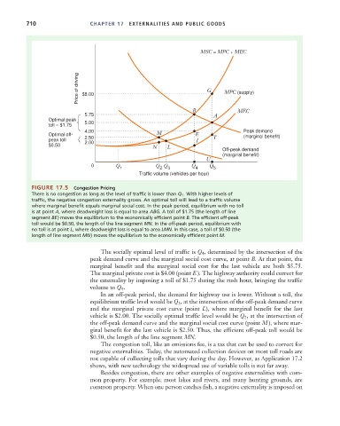
FIGURE 17.5 Congestion Pricing
There is no congestion as long as the level of traffic is lower than Q 1 . With higher levels of
traffic, the negative congestion externality grows. An optimal toll will lead to a traffic volume
where marginal benefit equals marginal social cost. In the peak period, equilibrium with no toll
is at point A, where deadweight loss is equal to area ABG. A toll of $1.75 (the length of line
segment BE) moves the equilibrium to the economically efficient point B. The efficient off-peak
toll would be $0.50, the length of the line segment MN. In the off-peak period, equilibrium with
no toll is at point L, where deadweight loss is equal to area LMN. In this case, a toll of $0.50 (the
length of line segment MN) moves the equilibrium to the economically efficient point M.

The socially optimal level of traffic is Q 4 , determined by the intersection of the
peak demand curve and the marginal social cost curve, at point B. At that point, the
marginal benefit and the marginal social cost for the last vehicle are both $5.75.
The marginal private cost is $4.00 (point E ). The highway authority could correct for
the externality by imposing a toll of $1.75 during the rush hour, bringing the traffic
volume to Q 4 .
In an off-peak period, the demand for highway use is lower. Without a toll, the
equilibrium traffic level would be Q 3 , at the intersection of the off-peak demand curve
and the marginal private cost curve (point L), where marginal benefit for the last
vehicle is $2.00. The socially optimal traffic level would be Q 2 , at the intersection of
the off-peak demand curve and the marginal social cost curve (point M ), where mar-
ginal benefit for the last vehicle is $2.50. Thus, the efficient off-peak toll would be
$0.50, the length of the line segment MN.
The congestion toll, like an emissions fee, is a tax that can be used to correct for
negative externalities. Today, the automated collection devices on most toll roads are
not capable of collecting tolls that vary during the day. However, as Application 17.2
shows, with new technology the widespread use of variable tolls is not far away.
Besides congestion, there are other examples of negative externalities with com-
mon property. For example, most lakes and rivers, and many hunting grounds, are
common property. When one person catches fish, a negative externality is imposed on