Page 83 - Microeconomics, Fourth Edition

c02demandandsupplyanalysis.qxd 6/14/10 1:39 PM Page 57

2.5 BACK-OF-THE-ENVELOPE CALCULATIONS 57

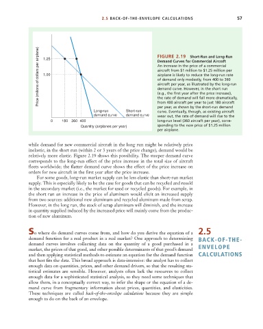
Price (milions of dollars per airplane) 1.25 FIGURE 2.19 Short-Run and Long-Run

Demand Curves for Commercial Aircraft
An increase in the price of a commercial
aircraft from $1 million to $1.25 million per
airplane is likely to reduce the long-run rate
1.00
of demand only modestly, from 400 to 360
aircraft per year, as illustrated by the long-run
demand curve. However, in the short run
(e.g., the first year after the price increase),
the rate of demand will fall more dramatically,
from 400 aircraft per year to just 180 aircraft
per year, as shown by the short-run demand
Long-run Short-run curve. Eventually, though, as existing aircraft
demand curve demand curve wear out, the rate of demand will rise to the
0 180 360 400 long-run level (360 aircraft per year), corre-
Quantity (airplanes per year) sponding to the new price of $1.25 million
per airplane.

while demand for new commercial aircraft in the long run might be relatively price
inelastic, in the short run (within 2 or 3 years of the price change), demand would be
relatively more elastic. Figure 2.19 shows this possibility. The steeper demand curve
corresponds to the long-run effect of the price increase in the total size of aircraft
fleets worldwide; the flatter demand curve shows the effect of the price increase on
orders for new aircraft in the first year after the price increase.
For some goods, long-run market supply can be less elastic than short-run market
supply. This is especially likely to be the case for goods that can be recycled and resold
in the secondary market (i.e., the market for used or recycled goods). For example, in
the short run an increase in the price of aluminum would elicit an increased supply
from two sources: additional new aluminum and recycled aluminum made from scrap.
However, in the long run, the stock of scrap aluminum will diminish, and the increase
in quantity supplied induced by the increased price will mainly come from the produc-
tion of new aluminum.

So where do demand curves come from, and how do you derive the equation of a 2.5
demand function for a real product in a real market? One approach to determining BACK-OF-THE-
demand curves involves collecting data on the quantity of a good purchased in a
market, the prices of that good, and other possible determinants of that good’s demand ENVELOPE
and then applying statistical methods to estimate an equation for the demand function CALCULATIONS
that best fits the data. This broad approach is data-intensive: the analyst has to collect
enough data on quantities, prices, and other demand drivers, so that the resulting sta-
tistical estimates are sensible. However, analysts often lack the resources to collect
enough data for a sophisticated statistical analysis, so they need some techniques that
allow them, in a conceptually correct way, to infer the shape or the equation of a de-
mand curve from fragmentary information about prices, quantities, and elasticities.
These techniques are called back-of-the-envelope calculations because they are simple
enough to do on the back of an envelope.