Page 84 - Microeconomics, Fourth Edition

c02demandandsupplyanalysis.qxd 6/14/10 1:39 PM Page 58

58 CHAPTER 2 DEMAND AND SUPPLY ANALYSIS
FITTING LINEAR DEMAND CURVES USING QUANTITY,
PRICE, AND ELASTICITY INFORMATION

Often, you can obtain information on the prevailing or typical prices and quantities
within a particular market as well as estimates of the price elasticity of demand in that
market. These estimates might come from statistical studies (this is where the elasticities
in Tables 2.1, 2.2, and 2.3 came from) or the judgments of informed observers (e.g.,
industry participants, investment analysts, consultants). If you assume as a rough approx-
imation that the equation of the demand curve is linear (i.e., Q a b P), you can then
derive the equation of this linear demand (i.e., the values of a and b) from these three
pieces of information (prevailing price, prevailing quantity, and estimated elasticity).
The approach to fitting a linear demand curve to quantity, price, and elasticity
data proceeds as follows. Suppose Q* and P* are the known values of quantity and
price in this market, and Q, P is the estimated value of the price elasticity of demand.
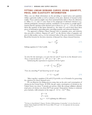
Recall the formula for the price elasticity of demand for a linear demand function.

P*
Q, P b (2.7)
Q*

Solving equation (2.7) for b yields

Q*
b Q, P (2.8)
P*

To solve for the intercept a, we note that Q* and P* must be on the demand curve.
Thus, it must be that Q* a bP*, or a Q* bP*.
Substituting the expression in equation (2.8) for b gives

Q*
a Q* a Q, P b P*
P*

Then, by canceling P* and factoring out Q*, we get

a (1 Q, P )Q* (2.9)

Taken together, equations (2.8) and (2.9) provide a set of formulas for generating
the equation of a linear demand curve.
We can illustrate the fitting process using data on the price and consumption of
chicken in the United States. In 1990, the per capita consumption of chicken in the
United States was about 70 pounds per person, while the average inflation-adjusted
retail price of chicken was about $0.70 per pound. Demand for chicken is relatively
price inelastic, with estimates in the range of 0.5 to 0.6. 20 Thus,

Q* 70
P* 0.70
Q, P 0.55 (splitting the difference)

20 All data are from Richard T. Rogers, “Broilers: Differentiating a Commodity,” in Larry Duetsch, ed.,
Industry Studies (Englewood Cliffs, NJ: Prentice Hall, 1993), pp. 3–32. See especially the data summa-
rized on pp. 4–6.