Page 85 - Microeconomics, Fourth Edition

c02demandandsupplyanalysis.qxd 6/14/10 1:39 PM Page 59

2.5 BACK-OF-THE-ENVELOPE CALCULATIONS 59

$2.00

Price (dollars per pound) $1.50 Observed price

$1.00
and quantity
$0.70
$0.50
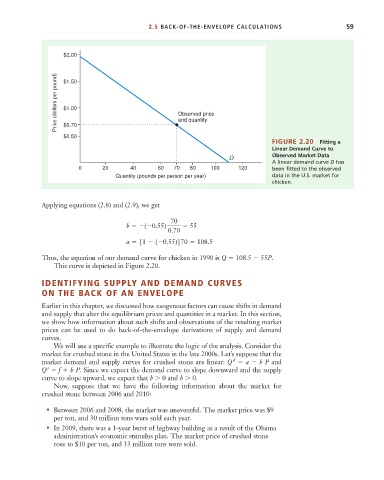
FIGURE 2.20 Fitting a
Linear Demand Curve to
D Observed Market Data
A linear demand curve D has
0 20 40 60 70 80 100 120 been fitted to the observed
Quantity (pounds per person per year) data in the U.S. market for
chicken.

Applying equations (2.8) and (2.9), we get

70
b ( 0.55) 55
0.70
a [1 ( 0.55)]70 108.5

Thus, the equation of our demand curve for chicken in 1990 is Q 108.5 55P.
This curve is depicted in Figure 2.20.

IDENTIFYING SUPPLY AND DEMAND CURVES
ON THE BACK OF AN ENVELOPE

Earlier in this chapter, we discussed how exogenous factors can cause shifts in demand
and supply that alter the equilibrium prices and quantities in a market. In this section,
we show how information about such shifts and observations of the resulting market
prices can be used to do back-of-the-envelope derivations of supply and demand
curves.
We will use a specific example to illustrate the logic of the analysis. Consider the
market for crushed stone in the United States in the late 2000s. Let’s suppose that the
d
market demand and supply curves for crushed stone are linear: Q a b P and
s
Q f h P. Since we expect the demand curve to slope downward and the supply
curve to slope upward, we expect that b
0 and h
0.
Now, suppose that we have the following information about the market for
crushed stone between 2006 and 2010:

• Between 2006 and 2008, the market was uneventful. The market price was $9
per ton, and 30 million tons were sold each year.
• In 2009, there was a 1-year burst of highway building as a result of the Obama
administration’s economic stimulus plan. The market price of crushed stone
rose to $10 per ton, and 33 million tons were sold.