Page 442 - Economics

CONFIRMING PAGES

374 CHAPTER NINETEEN APPENDIX

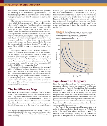
possesses the combination will substitute one good for (labeled I in Figure 3 ) reflects combinations of A and B
3
the other (say, B for A) to remain equally satisfied. The that yield more utility than I . Each curve to the left of I
3
3
diminishing slope of the indifference curve means that the reflects less total utility than I . As we move out from the
3
willingness to substitute B for A diminishes as more of B is origin, each successive indifference curve represents a
obtained. higher level of utility. To demonstrate this fact, draw a line
The rationale for this convexity—that is, for a dimin- in a northeasterly direction from the origin; note that its
ishing MRS—is that a consumer’s subjective willingness to points of intersection with successive curves entail larger
substitute B for A (or A for B) will depend on the amounts amounts of both A and B and therefore higher levels of
of B and A he or she has to begin with. Consider the table total utility.
and graph in Figure 2 again, beginning at point j . Here, in
relative terms, the consumer has a substantial amount of A
FIGURE 3 An indifference map. An indifference map is a
and very little of B. Within this combination, a unit of B is set of indifference curves. Curves farther from the origin indicate higher
very valuable (that is, its marginal utility is high), while a levels of total utility. Thus any combination of products A and B
represented by a point on I 4 has greater total utility than any combination
unit of A is less valuable (its marginal utility is low). The
of A and B represented by a point on I 3 , I 2 , or I 1 .
consumer will then be willing to give up a substantial
amount of A to get, say, 2 more units of B. In this case,
the consumer is willing to forgo 6 units of A to get 2 more 12
6 _
units of B; the MRS is , or 3, for the jk segment of the
2
curve.
But at point k the consumer has less A and more B. 10
Here A is somewhat more valuable, and B less valuable,
“at the margin.” In a move from point k to point l, the 8
consumer is willing to give up only 2 units of A to get 2 Quantity of A
2 _
more units of B, so the MRS is only , or 1. Having still 6
2
less of A and more of B at point l, the consumer is willing
to give up only 1 unit of A in return for 2 more units of B 4
1 _
1
and the MRS falls to between l and m . I 4
2
In general, as the amount of B increases, the marginal 2 I 3
utility of additional units of B decreases . Similarly, as the
I 2
quantity of A decreases, its marginal utility increases . In Fig- I 1
ure 2 we see that in moving down the curve, the consumer 0 2 4 6 8 10 12
will be willing to give up smaller and smaller amounts of A Quantity of B
to offset acquiring each additional unit of B. The result is
a curve with a diminishing slope, a curve that is convex to
the origin. The MRS declines as one moves southeast Equilibrium at Tangency
along the indifference curve. Since the axes in Figures 1 and 3 are identical, we can su-
perimpose a budget line on the consumer’s indifference
map, as shown in Figure 4 . By definition, the budget line
The Indifference Map indicates all the combinations of A and B that the con-
The single indifference curve of Figure 2 reflects some sumer can attain with his or her money income, given
constant (but unspecified) level of total utility or satisfac- the prices of A and B. Of these attainable combinations,
tion. It is possible and useful to sketch a whole series of the consumer will prefer the combination that yields the
indifference curves or an indifference map, as shown in greatest satisfaction or utility. Specifically, the utility-max-
Figure 3 . Each curve reflects a different level of total util- imizing combination will be the combination lying on the
ity and therefore never crosses another indifference curve. highest attainable indifference curve. It is called the con-
Specifically, each curve to the right of our original curve sumer’s equilibrium position .
In Figure 4 the consumer’s equilibrium position is at
. Why not
point X, where the budget line is tangent to I 3
1 MRS declines continuously between j and k, k and l, and l and m. Our
2
numerical values for MRS relate to the curve segments between points point Y? Because Y is on a lower indifference curve, I . By
and are not the actual values of the MRS at each point. For example, the moving “down” the budget line—by shifting dollars from
2 _
MRS at point l is . purchases of A to purchases of B—the consumer can attain
3

6/3/06 12:53:25 PM
mcc26632_ch19_359-377.indd 374 6/3/06 12:53:25 PM
mcc26632_ch19_359-377.indd 374