Page 444 - Economics

CONFIRMING PAGES

376 CHAPTER NINETEEN APPENDIX

curve theory does not require that the consumer specify how things equal,” since only the price of B was changed (the
much more (or less) satisfaction will be realized. price of A and the consumer’s money income and tastes re-
When we compare the equilibrium situations in the mained constant). But, in this case, we have derived the de-
two theories, we find that in the indifference curve analy- mand curve without resorting to the questionable
sis the MRS equals P B P A at equilibrium; however, in the assumption that consumers can measure utility in units
marginal-utility approach the ratio of marginal utilities called “utils.” In this indifference curve approach, consum-
equals P P . We therefore deduce that at equilibrium the ers simply compare combinations of products A and B and
A
B
MRS is equivalent in the marginal-utility approach to the determine which combination they prefer, given their in-
ratio of the marginal utilities of the last purchased units of comes and the prices of the two products.
2
the two products.
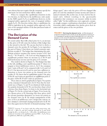
FIGURE 5 Deriving the demand curve. (a) When the price of
The Derivation of the product B is increased from $1 to $1.50, the equilibrium position moves from X
to X', decreasing the quantity of product B demanded from 6 to 3 units. (b) The
Demand Curve demand curve for product B is determined by plotting the $1–6-unit and the
$1.50–3-unit price-quantity combinations for product B.
We noted earlier that with a fixed price for A, an increase
in the price of B will cause the bottom of the budget line 12
to fan inward to the left. We can use that fact to derive a
demand curve for product B. In Figure 5 a we reproduce 10
the part of Figure 4 that shows our initial consumer equi-
librium at point X . The budget line determining this equi- 8
librium position assumes that money income is $12 and P B = $1
$1.50 and P $1. Let’s see what happens to the
that P A B Quantity of A 6
equilibrium position when we increase P to $1.50 and
B
hold both money income and the price of A constant. X X
4
The result is shown in Figure 5 a. The budget line fans
to the left, yielding a new equilibrium point X' where it is I 3
tangent to lower indifference curve I . At X ' the consumer 2
2
buys 3 units of B and 5 of A, compared with 4 of A and 6 of P B = $1.50 I 2
B at X. Our interest is in B, and we now have sufficient in-
formation to locate two points on the demand curve for 0 2 4 6 8 10 12
product B. We know that at equilibrium point X the price Quantity of B
of B is $1 and 6 units are purchased; at equilibrium point X' (a)
the price of B is $1.50 and 3 units are purchased. Two equilibrium positions
These data are shown graphically in Figure 5 b as points
on the consumer’s demand curve for B. Note that the hori-
zontal axes of Figure 5 a and 5b are identical; both measure
the quantity demanded of B. We can therefore drop vertical
reference lines from Figure 5 a down to the horizontal axis
of Figure 5 b. On the vertical axis of Figure 5 b we locate the
two chosen prices of B. Knowing that these prices yield $1.50
the relevant quantities demanded, we locate two points on Price of B
the demand curve for B. By simple manipulation of the
price of B in an indifference curve–budget line context, we 1.00
have obtained a downward-sloping demand curve for B. We
have thus again derived the law of demand assuming “other .50
D B
2 Technical footnote: If we begin with the utility-maximizing rule,
MU A P A MU B P B , and then multiply through by P B and divide 0 1 2 3 4 5 6 7 8 9 10 11 12
through by MU A , we obtain P B P A MU B MU A . In indifference curve Quantity of B
analysis we know that at the equilibrium position MRS P B P A . Hence, (b)
at equilibrium, MRS also equals MU B MU A . The demand curve for product B

6/3/06 12:53:26 PM
mcc26632_ch19_359-377.indd 376
mcc26632_ch19_359-377.indd 376 6/3/06 12:53:26 PM