Page 88 - ISCI’2017

The power of different t-sequences sets of l-bit values is equal to 2 , and each of these sequences
tl
with the probability (9) appear at the output of the round key schedule construction at least once. I. e.

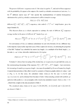
for 2 k different master keys K ()x that specify the implementations of random homogenious

substitution the cyclic key schedule construction it will be formed in average
k
N ( , , ) 2 (1k lt = tl − P (2 ,0, ))t

1
−
different K () x = {K 1 () x ,K 2 () x ,...,K t () x } sequences, what under(1 2 )− l − 2 l ≈ e simplification gives the
рк
target formula (8).
This theorem allows us to obtain expression to estimate the ratio of different K ()x sequences
рк

average number to the power of different K ()x master keys set:
−
( ,, )
N k lt k   1  2 k tl  k tl
−
k lt
δ ( , , ) = = 2 tl k (1 (1 2 ) ) ≈ 2 tl k 1     − ≈ 2 tl k ( 1− (0,37 ) 2 ) (10)
2
tl
−
−
−
−−
−
2 k   e  
 
δ
k lt
For convenience of ( ,, ) relations calculations we can write formula (10) in a different way.
In the majority of practically important cases of block cipher (for instance, in estimating the properties
of the BSC "Kalyna" key schedule) the master key length k is a multiple of the block length l, i.e.
the ratio k = ml is true, what after substitution in (10) it gives
  1  2 ( l m t − )  ( l m t − )
tl
−
−
−
−−
−
δ (mllt = 2 ( lt m ) (1 (1 2 ) 2 ml ) ≈ 2 ( lt m ) 1     − ≈ 2 ( lt m ) ( 1− (0,37 ) 2 ) . (11)
, , )
  e  
 
Formula (11) shows that increasing of the multiplicity m is equivalent, in a probabilistic sense, to
the corresponding decreasing of the sequence K () x = {K 1 () x ,K 2 () x ,...,K t () x } length t. And conversely,
рк
the increasing of round keys sequence length t decreases the probability (9) as well master key length.
A typical demonstration of this effect would be symmetry of function graphs relative to values l and
,, )
k (Fig. 2, 3). In this sense, the calculated values δ (mllt for the case l ∈ {16,32} and
, mt ∈ {1,2,4,8,16} can be obtained from the data in Table 1 when selecting column with symbols ml
and rows with symbols tl . As an example, table 2 shows the calculated values1 (mlltδ ,, ) for l = 32

, which fully comply to the data presented in Table 1.

}
}
}
The calculated values (mlltδ ,, ) for cases l ∈ {64,128,256 , m∈ {1,2,4,8 and t ∈ {1,2,4,8,16
are shown in Table 3 .

1 Values (mlltδ ,, ) in tables 2-4 are calculated using simplified formula е (mlltδ ,, ) ≈ 2 ( lt m− ) ( 1 e− − 2 ( l m t− ) )
88