Page 106 - Fiber Optic Communications Fund

Optical Fiber Transmission 87

The field envelope may be written as

s(t, z)= A(t, z) exp [i(t, z)]. (2.267)
The instantaneous frequency deviation from the carrier frequency is given by Eq. (2.165) as

d
(t, z)=− . (2.268)
dt
At the fiber input, we have
2
t C
(t, 0)=− . (2.269)
2T 2
0
So, the instantaneous frequency deviation from the carrier frequency is
Ct
(t, 0)= . (2.270)
T 2
0
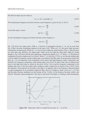
Fig. 2.40 shows the output pulse width as a function of propagation distance L. As can be seen from
Eq. (2.266), the pulse broadening depends on the sign of C. When C ≥ 0, the pulse width increases
2 2
with distance monotonically. When C < 0, the first term within the square bracket of Eq. (2.266) becomes
2
less than unity and, therefore, the output pulse width can be less than the input pulse width for certain
distances. Fig. 2.40 shows that the pulse undergoes compression initially for C = 4 and < 0. The physical
2
explanation for pulse compression is as follows. When C > 0, from Eq. (2.270), we see that the leading edge
is down-shifted in frequency and the trailing edge is up-shifted at the fiber input. In an anomalous dispersion
fiber ( < 0), low-frequency (red) components travel slower than high-frequency (blue) components and,
2
therefore, the frequency components at the leading edge travel slowly. In other words, they are delayed and
move to the right (later time) as shown by the arrow in Fig. 2.41(a), and the frequency components at the
leading edge move to the left (earlier time), leading to pulse compression as shown in Fig. 2.41(b). Since
the frequency chirp imposed on the pulse at the input is of opposite sign to the frequency chirp developed
via pulse propagation in an anomalous dispersion fiber, these two frequency chirps cancel at L = 12.5km
and the pulse becomes unchirped (see the bottom of Fig. 2.41(b)). At this distance, the pulse width is the
shortest. Thereafter, pulse propagation is the same as discussed in Example 2.6, leading to pulse broadening.

2
Figure 2.40 Output pulse width of a chirped Gaussian pulse. =−21 ps /km.
2